12.2: Calculation of Volumes in Higher Dimensions

Three Dimensions

Both the Monte Carlo method and Riemann sum used to estimate the area of region \(D\) in two dimensions trivially extends to higher dimensions. Let us consider their applications in three dimensions.

Monte Carlo

Now, we sample \(\left(X_{1}, X_{2}, X_{3}\right)\) uniformly from a parallelepiped \(R=\left[a_{1}, b_{1}\right] \times\left[a_{2}, b_{2}\right] \times\left[a_{3}, b_{3}\right]\), where the \(X_{i}\) ’s are mutually independent. Then, we assign a Bernoulli random variable according to whether \(\left(X_{1}, X_{2}, X_{3}\right)\) is inside or outside \(D\) as before, i.e. \[B= \begin{cases}1, & \left(X_{1}, X_{2}, X_{3}\right) \in D \\ 0, & \text { otherwise }\end{cases}\] Recall that the convergence of the sample mean to the true value - in particular the convergence of the confidence interval - is related to the Bernoulli random variable and not the \(X_{i}\) ’s. Thus, even in three dimensions, we still expect the error to converge as \(N^{-1 / 2}\), where \(N\) is the size of the sample.

Riemann Sum

For simplicity, let us assume the parallelepiped is a cube, i.e. \(a=a_{1}=a_{2}=a_{3}\) and \(b=b_{1}=b_{2}=b_{3}\). We consider a grid of \(N\) points centered in little cubes of size \[h^{3}=\frac{b-a}{N},\] such that \(N h^{3}=V_{R}\). Extending the two-dimensional case, we estimate the volume of the region \(D\) according to \[\frac{\widehat{V}_{D}^{\mathrm{Rie}}}{V_{R}}=\frac{\text { number of points in } D}{N} .\] However, unlike the Monte Carlo method, the error calculation is dependent on the dimension. The error is given by \[\begin{aligned} \text { error } & \approx(\text { number of cubes that intersect } D) \cdot h^{3} \\ & \approx\left(\text { surface area of } D / h^{2}\right) \cdot h^{3} \\ & \approx h \approx N^{-1 / 3} . \end{aligned}\] Note that the convergence rate has decreased from \(N^{-1 / 2}\) to \(N^{-1 / 3}\) in going from two to three dimensions.

Example 12.2.1 Integration of a sphere

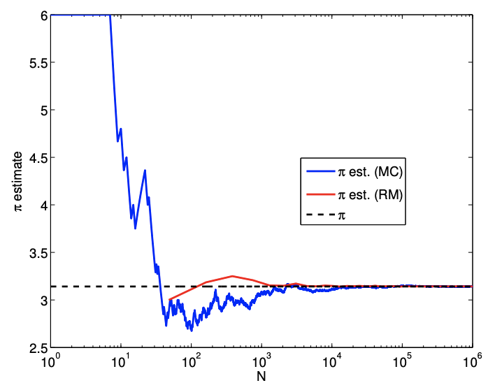
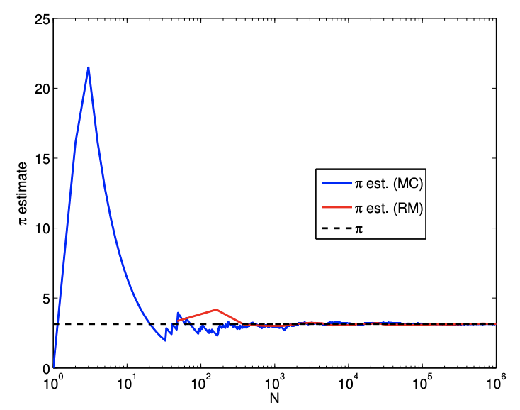
Let us consider a problem of finding the volume of a unit \(1 / 8\) th sphere lying in the first octant. We sample from a unit cube \[R=[0,1] \times[0,1] \times[0,1]\] having a volume of \(V_{R}=1.0\). As in the case of circle in two dimensions, we can perform simple in/out check by measuring the distance of the point from the origin; i.e the Bernoulli variable is assigned according to \[b_{n}=\left\{\begin{array}{ll} 1, & \sqrt{x_{1}^{2}+x_{2}^{2}+x_{3}^{2}} \leq 1 \\ 0, & \text { otherwise } \end{array} .\right.\] The result of estimating the value of \(\pi\) based on the estimate of the volume of the \(1 / 8\) th sphere is shown in Figure 12.7. (The raw estimated volume of the 1/8th sphere is scaled by 6.) As expected

(a) value

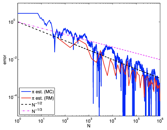
(b) error

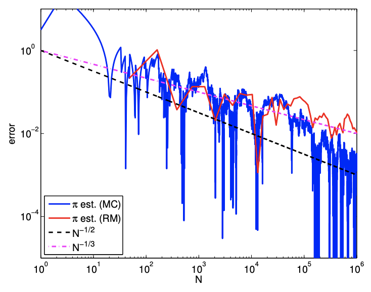
Figure 12.7: Convergence of the \(\pi\) estimate using the volume of a sphere.

both the Monte Carlo method and the Riemann sum converge to the correct value. In particular, the Monte Carlo method converges at the expected rate of \(N^{-1 / 2}\). The Riemann sum, on the other hand, converges at a faster rate than the expected rate of \(N^{-1 / 3}\). This superconvergence is due to the symmetry in the tetrahedralization used in integration and the volume of interest. This does not contradict our a priori analysis, because the analysis tells us the asymptotic convergence rate for the worst case. The following example shows that the asymptotic convergence rate of the Riemann sum for a general geometry is indeed \(N^{-1 / 2}\).

Example 12.2.2 Integration of a parallelpiped

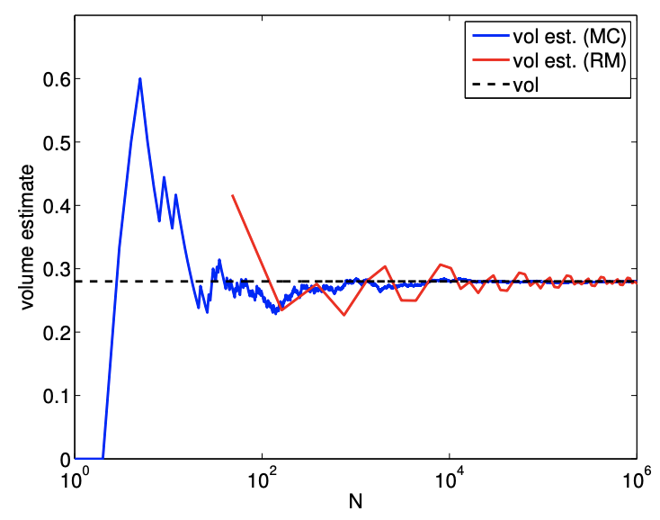
Let us consider a simpler example of finding the volume of a parallelpiped described by \[D=[0.1,0.9] \times[0.2,0.7] \times[0.1,0.8] .\] The volume of the parallelpiped is \(V_{D}=0.28\).

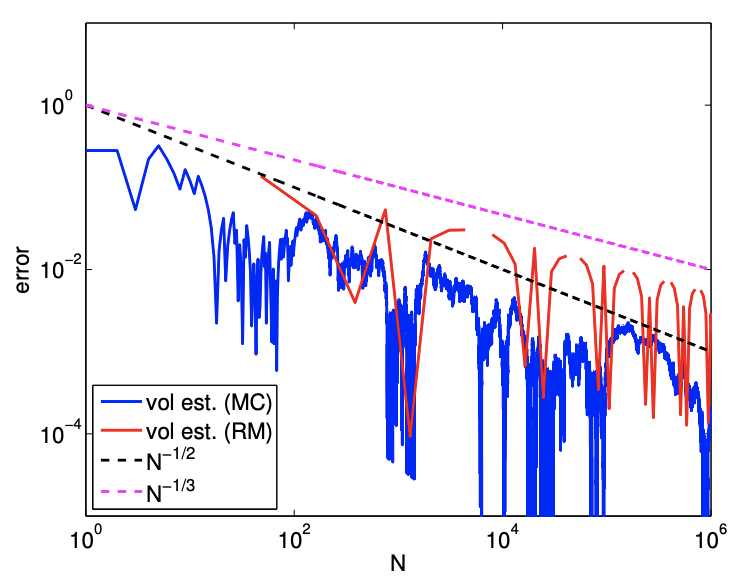
Figure \(12.8\) shows the result of the integration. The figure shows that the convergence rate of the Riemann sum is \(N^{-1 / 3}\), which is consistent with the a priori analysis. On the other hand, the Monte Carlo method performs just as well as it did in two dimension, converging at the rate of \(N^{-1 / 2}\). In particular, the Monte Carlo method performs noticeably better than the Riemann sum for large values of \(N\).

Example 12.2.3 Integration of a complex volume

Let us consider a more general geometry, with the domain defined in the spherical coordinate as \[D=\left\{(r, \theta, \phi): r \leq \sin (\theta)\left(\frac{2}{3}+\frac{1}{3} \cos (40 \phi)\right), 0 \leq \theta \leq \frac{\pi}{2}, 0 \leq \phi \leq \frac{\pi}{2}\right\} .\] The volume of the region is given by \[V_{D}=\int_{\phi=0}^{\pi / 2} \int_{\theta=0}^{\pi / 2} \int_{r=0}^{\sin (\theta)\left(\frac{2}{3}+\frac{1}{3} \cos (40 \phi)\right)} r^{2} \sin (\theta) d r d \theta d \phi=\frac{88}{2835} \pi .\]

(a) value

(b) error

Figure 12.8: Area of a parallelepiped.

(a) value

(b) error

Figure 12.9: Convergence of the \(\pi\) estimate using a complex three-dimensional integration.

Thus, we can estimate the value of \(\pi\) by first estimating the volume using Monte Carlo or Riemann sum, and then multiplying the result by \(2835 / 88\).

Figure \(12.9\) shows the result of performing the integration. The figure shows that the convergence rate of the Riemann sum is \(N^{-1 / 3}\), which is consistent with the a priori analysis. On the other hand, the Monte Carlo method performs just as well as it did for the simple sphere case.

General \(d\)-Dimensions

Let us generalize our analysis to the case of integrating a general \(d\)-dimensional region. In this case, the Monte Carlo method considers a random \(d\)-vector, \(\left(X_{1}, \ldots, X_{d}\right)\), and associate with the vector a Bernoulli random variable. The convergence of the Monte Carlo integration is dependent on the Bernoulli random variables and not directly affected by the random vector. In particular, the Monte Carlo method is oblivious to the length of the vector, \(d\), i.e. the dimensionality of the space. Because the standard deviation of the binomial distribution scales as \(N^{-1 / 2}\), we still expect the Monte Carlo method to converge at the rate of \(N^{-1 / 2}\) regardless of \(d\). Thus, Monte Carlo methods do not suffer from so-called curse of dimensionality, in which a method becomes intractable with increase of the dimension of the problem.

On the other hand, the performance of the Riemann sum is a function of the dimension of the space. In a \(d\)-dimensional space, each little cube has the volume of \(N^{-1}\), and there are \(N^{\frac{d-1}{d}}\) cube that intersect the boundary of \(D\). Thus, the error scales as \[\text { error } \approx N^{\frac{d-1}{d}} N^{-1}=N^{-1 / d} .\] The convergence rate worsens with the dimension, and this is an example of the curse of dimensionality. While the integration of a physical volume is typically limited to three dimensions, there are many instances in science and engineering where a higher-dimensional integration is required.

Example 12.2.4 integration over a hypersphere

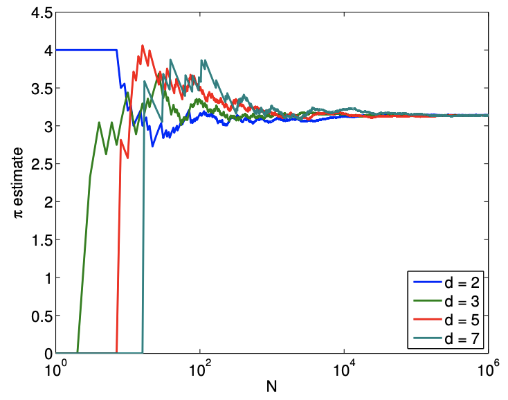
To demonstrate that the convergence of Monte Carlo method is independent of the dimension, let us consider integration of a hypersphere in \(d\)-dimensional space. The volume of \(d\)-sphere is given by \[V_{D}=\frac{\pi^{d / 2}}{\Gamma(n / 2+1)} r^{d},\] where \(\Gamma\) is the gamma function. We can again use the integration of a \(d\)-sphere to estimate the value of \(\pi\).

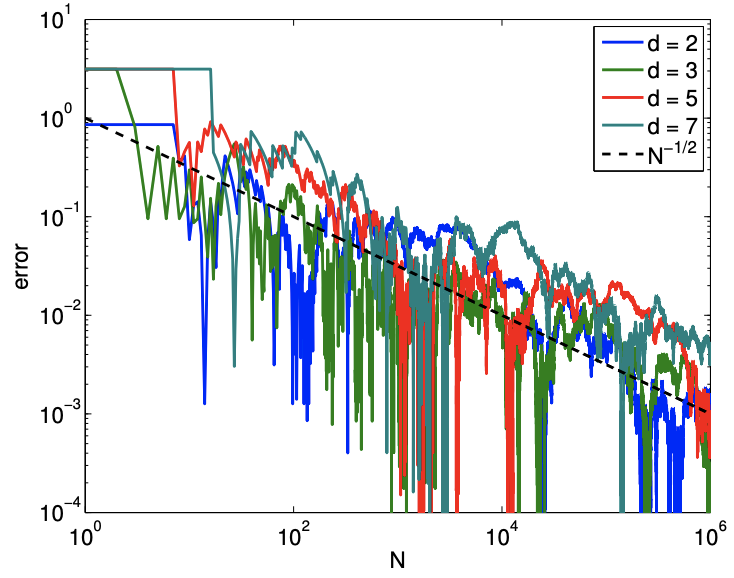
The result of estimating the \(d\)-dimensional volume is shown in Figure \(12.10\) for \(d=2,3,5,7\). The error convergence plot shows that the method converges at the rate of \(N^{-1 / 2}\) for all \(d\). The result confirms that Monte Carlo integration is a powerful method for integrating functions in higher-dimensional spaces.

(a) value

(b) error

Figure 12.10: Convergence of the \(\pi\) estimate using the Monte Carlo method on \(d\)-dimensional hyperspheres.