17.1: Data Fitting in Absence of Noise and Bias

We motivate our discussion by reconsidering the friction coefficient example of Chapter 15 . We recall that, according to Amontons, the static friction, \(F_{\mathrm{f}, \text { static }}\), and the applied normal force, \(F_{\text {normal, applied, }}\), are related by \[F_{\mathrm{f}, \text { static }} \leq \mu_{\mathrm{s}} F_{\text {normal, applied }}\] here \(\mu_{\mathrm{s}}\) is the coefficient of friction, which is only dependent on the two materials in contact. In particular, the maximum static friction is a linear function of the applied normal force, i.e. \[F_{\mathrm{f}, \text { static }}^{\max }=\mu_{\mathrm{s}} F_{\text {normal, applied }} .\] We wish to deduce \(\mu_{\mathrm{s}}\) by measuring the maximum static friction attainable for several different values of the applied normal force.

Our approach to this problem is to first choose the form of a model based on physical principles and then deduce the parameters based on a set of measurements. In particular, let us consider a simple affine model \[y=Y_{\text {model }}(x ; \beta)=\beta_{0}+\beta_{1} x .\] The variable \(y\) is the predicted quantity, or the output, which is the maximum static friction \(F_{\mathrm{f}, \text { static }}^{\max }\). The variable \(x\) is the independent variable, or the input, which is the maximum normal force \(F_{\text {normal, applied }}\). The function \(Y_{\text {model }}\) is our predictive model which is parameterized by a parameter \(\beta=\left(\beta_{0}, \beta_{1}\right)\). Note that Amontons’ law is a particular case of our general affine model with \(\beta_{0}=0\) and \(\beta_{1}=\mu_{\mathrm{s}}\). If we take \(m\) noise-free measurements and Amontons’ law is exact, then we expect \[F_{\mathrm{f}, \text { static } i}^{\max }=\mu_{\mathrm{S}} F_{\text {normal, applied } i}, \quad i=1, \ldots, m\] The equation should be satisfied exactly for each one of the \(m\) measurements. Accordingly, there is also a unique solution to our model-parameter identification problem \[y_{i}=\beta_{0}+\beta_{1} x_{i}, \quad i=1, \ldots, m,\] with the solution given by \(\beta_{0}^{\text {true }}=0\) and \(\beta_{1}^{\text {true }}=\mu_{\mathrm{s}}\).

Because the dependency of the output \(y\) on the model parameters \(\left\{\beta_{0}, \beta_{1}\right\}\) is linear, we can write the system of equations as a \(m \times 2\) matrix equation \[\underbrace{\left(\begin{array}{cc} 1 & x_{1} \\ 1 & x_{2} \\ \vdots & \vdots \\ 1 & x_{m} \end{array}\right)}_{X} \underbrace{\left(\begin{array}{c} \beta_{0} \\ \beta_{1} \end{array}\right)}_{\beta}=\underbrace{\left(\begin{array}{c} y_{1} \\ y_{2} \\ \vdots \\ y_{m} \end{array}\right)}_{Y},\] or, more compactly, \[X \beta=Y .\] Using the row interpretation of matrix-vector multiplication, we immediately recover the original set of equations, \[X \beta=\left(\begin{array}{c} \beta_{0}+\beta_{1} x_{1} \\ \beta_{0}+\beta_{1} x_{2} \\ \vdots \\ \beta_{0}+\beta_{1} x_{m} \end{array}\right)=\left(\begin{array}{c} y_{1} \\ y_{2} \\ \vdots \\ y_{m} \end{array}\right)=Y .\] Or, using the column interpretation, we see that our parameter fitting problem corresponds to choosing the two weights for the two \(m\)-vectors to match the right-hand side, \[X \beta=\beta_{0}\left(\begin{array}{c} 1 \\ 1 \\ \vdots \\ 1 \end{array}\right)+\beta_{1}\left(\begin{array}{c} x_{1} \\ x_{2} \\ \vdots \\ x_{m} \end{array}\right)=\left(\begin{array}{c} y_{1} \\ y_{2} \\ \vdots \\ y_{m} \end{array}\right)=Y .\] We emphasize that the linear system \(X \beta=Y\) is overdetermined, i.e., more equations than unknowns \((m>n)\). (We study this in more detail in the next section.) However, we can still find a solution to the system because the following two conditions are satisfied:

Unbiased: Our model includes the true functional dependence \(y=\mu_{\mathrm{s}} x\), and thus the model is capable of representing this true underlying functional dependence. This would not be the case if, for example, we consider a constant model \(y(x)=\beta_{0}\) because our model would be incapable of representing the linear dependence of the friction force on the normal force. Clearly the assumption of no bias is a very strong assumption given the complexity of the physical world.

Noise free: We have perfect measurements: each measurement \(y_{i}\) corresponding to the independent variable \(x_{i}\) provides the "exact" value of the friction force. Obviously this is again rather naïve and will need to be relaxed.

Under these assumptions, there exists a parameter \(\beta^{\text {true }}\) that completely describe the measurements, i.e. \[y_{i}=Y_{\text {model }}\left(x ; \beta^{\text {true }}\right), \quad i=1, \ldots, m .\] (The \(\beta^{\text {true }}\) will be unique if the columns of \(X\) are independent.) Consequently, our predictive model is perfect, and we can exactly predict the experimental output for any choice of \(x\), i.e. \[Y(x)=Y_{\text {model }}\left(x ; \beta^{\text {true }}\right), \quad \forall x,\] where \(Y(x)\) is the experimental measurement corresponding to the condition described by \(x\). However, in practice, the bias-free and noise-free assumptions are rarely satisfied, and our model is never a perfect predictor of the reality.

In Chapter 19 , we will develop a probabilistic tool for quantifying the effect of noise and bias; the current chapter focuses on developing a least-squares technique for solving overdetermined linear system (in the deterministic context) which is essential to solving these data fitting problems. In particular we will consider a strategy for solving overdetermined linear systems of the form \[B z=g,\] where \(B \in \mathbb{R}^{m \times n}, z \in \mathbb{R}^{n}\), and \(g \in \mathbb{R}^{m}\) with \(m>n\).

Before we discuss the least-squares strategy, let us consider another example of overdetermined systems in the context of polynomial fitting. Let us consider a particle experiencing constant acceleration, e.g. due to gravity. We know that the position \(y\) of the particle at time \(t\) is described by a quadratic function \[y(t)=\frac{1}{2} a t^{2}+v_{0} t+y_{0},\] where \(a\) is the acceleration, \(v_{0}\) is the initial velocity, and \(y_{0}\) is the initial position. Suppose that we do not know the three parameters \(a, v_{0}\), and \(y_{0}\) that govern the motion of the particle and we are interested in determining the parameters. We could do this by first measuring the position of the particle at several different times and recording the pairs \(\left\{t_{i}, y\left(t_{i}\right)\right\}\). Then, we could fit our measurements to the quadratic model to deduce the parameters.

The problem of finding the parameters that govern the motion of the particle is a special case of a more general problem: polynomial fitting. Let us consider a quadratic polynomial, i.e. \[y(x)=\beta_{0}^{\text {true }}+\beta_{1}^{\text {true }} x+\beta_{2}^{\text {true }} x^{2},\] where \(\beta^{\text {true }}=\left\{\beta_{0}^{\text {true }}, \beta_{1}^{\text {true }}, \beta_{2}^{\text {true }}\right\}\) is the set of true parameters characterizing the modeled phenomenon. Suppose that we do not know \(\beta^{\text {true }}\) but we do know that our output depends on the input \(x\) in a quadratic manner. Thus, we consider a model of the form \[Y_{\text {model }}(x ; \beta)=\beta_{0}+\beta_{1} x+\beta_{2} x^{2},\] and we determine the coefficients by measuring the output \(y\) for several different values of \(x\). We are free to choose the number of measurements \(m\) and the measurement points \(x_{i}, i=1, \ldots, m\). In particular, upon choosing the measurement points and taking a measurement at each point, we obtain a system of linear equations, \[y_{i}=Y_{\text {model }}\left(x_{i} ; \beta\right)=\beta_{0}+\beta_{1} x_{i}+\beta_{2} x_{i}^{2}, \quad i=1, \ldots, m,\] where \(y_{i}\) is the measurement corresponding to the input \(x_{i}\).

Note that the equation is linear in our unknowns \(\left\{\beta_{0}, \beta_{1}, \beta_{2}\right\}\) (the appearance of \(x_{i}^{2}\) only affects the manner in which data enters the equation). Because the dependency on the parameters is linear, we can write the system as matrix equation, \[\underbrace{\left(\begin{array}{c} y_{1} \\ y_{2} \\ \vdots \\ y_{m} \end{array}\right)}_{Y}=\underbrace{\left(\begin{array}{ccc} 1 & x_{1} & x_{1}^{2} \\ 1 & x_{2} & x_{2}^{2} \\ \vdots & \vdots & \vdots \\ 1 & x_{m} & x_{m}^{2} \end{array}\right)}_{X} \underbrace{\left(\begin{array}{c} \beta_{0} \\ \beta_{1} \\ \beta_{2} \end{array}\right)}_{\beta},\] or, more compactly, \[Y=X \beta .\] Note that this particular matrix \(X\) has a rather special structure - each row forms a geometric series and the \(i j\)-th entry is given by \(B_{i j}=x_{i}^{j-1}\). Matrices with this structure are called Vandermonde matrices.

As in the friction coefficient example considered earlier, the row interpretation of matrix-vector product recovers the original set of equation \[Y=\left(\begin{array}{c} y_{1} \\ y_{2} \\ \vdots \\ y_{m} \end{array}\right)=\left(\begin{array}{c} \beta_{0}+\beta_{1} x_{1}+\beta_{2} x_{1}^{2} \\ \beta_{0}+\beta_{1} x_{2}+\beta_{2} x_{2}^{2} \\ \vdots \\ \beta_{0}+\beta_{1} x_{m}+\beta_{2} x_{m}^{2} \end{array}\right)=X \beta .\] With the column interpretation, we immediately recognize that this is a problem of finding the three coefficients, or parameters, of the linear combination that yields the desired \(m\)-vector \(Y\), i.e. \[Y=\left(\begin{array}{c} y_{1} \\ y_{2} \\ \vdots \\ y_{m} \end{array}\right)=\beta_{0}\left(\begin{array}{c} 1 \\ 1 \\ \vdots \\ 1 \end{array}\right)+\beta_{1}\left(\begin{array}{c} x_{1} \\ x_{2} \\ \vdots \\ x_{m} \end{array}\right)+\beta_{2}\left(\begin{array}{c} x_{1}^{2} \\ x_{2}^{2} \\ \vdots \\ x_{m}^{2} \end{array}\right)=X \beta .\] We know that if have three or more non-degenerate measurements (i.e., \(m \geq 3\) ), then we can find the unique solution to the linear system. Moreover, the solution is the coefficients of the underlying polynomial, \(\left(\beta_{0}^{\text {true }}, \beta_{1}^{\text {true }}, \beta_{2}^{\text {true }}\right)\).

Example 17.1.1 A quadratic polynomial

Let us consider a more specific case, where the underlying polynomial is of the form \[y(x)=-\frac{1}{2}+\frac{2}{3} x-\frac{1}{8} c x^{2} .\] We recognize that \(y(x)=Y_{\text {model }}\left(x ; \beta^{\text {true }}\right)\) for \(Y_{\text {model }}(x ; \beta)=\beta_{0}+\beta_{1} x+\beta_{2} x^{2}\) and the true parameters \[\beta_{0}^{\text {true }}=-\frac{1}{2}, \quad \beta_{1}^{\text {true }}=\frac{2}{3}, \quad \text { and } \quad \beta_{2}^{\text {true }}=-\frac{1}{8} c\] The parameter \(c\) controls the degree of quadratic dependency; in particular, \(c=0\) results in an affine function.

First, we consider the case with \(c=1\), which results in a strong quadratic dependency, i.e., \(\beta_{2}^{\text {true }}=-1 / 8\). The result of measuring \(y\) at three non-degenerate points \((m=3)\) is shown in Figure \(17.1(\mathrm{a})\). Solving the \(3 \times 3\) linear system with the coefficients as the unknown, we obtain \[\beta_{0}=-\frac{1}{2}, \quad \beta_{1}=\frac{2}{3}, \quad \text { and } \quad \beta_{2}=-\frac{1}{8} .\]

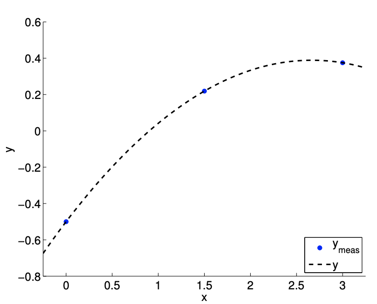
(a) \(m=3\)

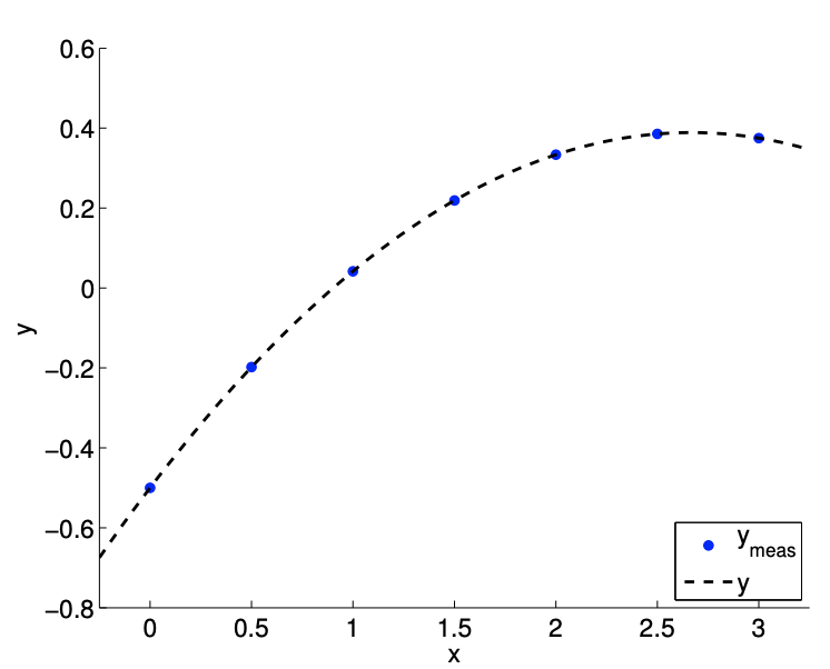
(b) \(m=7\)

Figure 17.1: Deducing the coefficients of a polynomial with a strong quadratic dependence.

Not surprisingly, we can find the true coefficients of the quadratic equation using three data points.

Suppose we take more measurements. An example of taking seven measurements \((m=7)\) is shown in Figure 17.1(b). We now have seven data points and three unknowns, so we must solve the \(7 \times 3\) linear system, i.e., find the set \(\beta=\left\{\beta_{0}, \beta_{1}, \beta_{2}\right\}\) that satisfies all seven equations. The solution to the linear system, of course, is given by \[\beta_{0}=-\frac{1}{2}, \quad \beta_{1}=\frac{2}{3}, \quad \text { and } \quad \beta_{2}=-\frac{1}{8} .\] The result is correct \(\left(\beta=\beta^{\text {true }}\right)\) and, in particular, no different from the result for the \(m=3\) case.

We can modify the underlying polynomial slightly and repeat the same exercise. For example, let us consider the case with \(c=1 / 10\), which results in a much weaker quadratic dependency of \(y\) on \(x\), i.e., \(\beta_{2}^{\text {true }}=-1 / 80\). As shown in Figure 17.1.1, we can take either \(m=3\) or \(m=7\) measurements. Similar to the \(c=1\) case, we identify the true coefficients, \[\beta_{0}=-\frac{1}{2}, \quad \beta_{1}=\frac{2}{3}, \quad \text { and } \beta_{2}=-\frac{1}{80},\] using the either \(m=3\) or \(m=7\) (in fact using any three or more non-degenerate measurements).

In the friction coefficient determination and the (particle motion) polynomial identification problems, we have seen that we can find a solution to the \(m \times n\) overdetermined system \((m>n)\) if

(a) our model includes the underlying input-output functional dependence - no bias;

(b) and the measurements are perfect - no noise.

As already stated, in practice, these two assumptions are rarely satisfied; i.e., models are often (in fact, always) incomplete and measurements are often inaccurate. (For example, in our particle motion model, we have neglected friction.) We can still construct a \(m \times n\) linear system \(B z=g\) using our model and measurements, but the solution to the system in general does not exist. Knowing that we cannot find the "solution" to the overdetermined linear system, our objective is

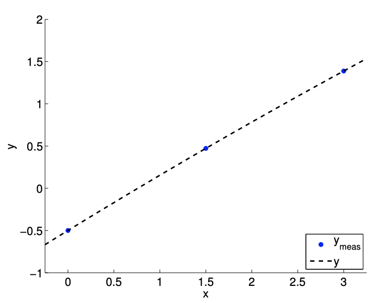
(a) \(m=3\)

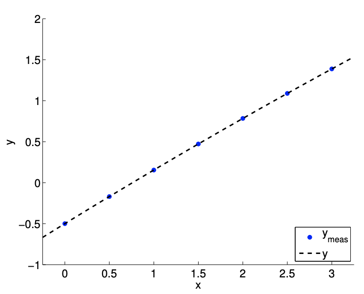
(b) \(m=7\)

Figure 17.2: Deducing the coefficients of a polynomial with a weak quadratic dependence.

to find a solution that is "close" to satisfying the solution. In the following section, we will define the notion of "closeness" suitable for our analysis and introduce a general procedure for finding the "closest" solution to a general overdetermined system of the form \[B z=g,\] where \(B \in \mathbb{R}^{m \times n}\) with \(m>n\). We will subsequently address the meaning and interpretation of this (non-) solution.