17.3: Least Squares

Measures of Closeness

In the previous section, we observed that it is in general not possible to find a solution to an overdetermined system. Our aim is thus to find \(z\) such that \(B z\) is "close" to \(g\), i.e., \(z\) such that \[B z \approx g,\] for \(B \in \mathbb{R}^{m \times n}, m>n\). For convenience, let us introduce the residual function, which is defined as \[r(z) \equiv g-B z .\] Note that \[r_{i}=g_{i}-(B z)_{i}=g_{i}-\sum_{j=1}^{n} B_{i j} z_{j}, \quad i=1, \ldots, m .\] Thus, \(r_{i}\) is the "extent" to which \(i\)-th equation \((B z)_{i}=g_{i}\) is not satisfied. In particular, if \(r_{i}(z)=0\), \(i=1, \ldots, m\), then \(B z=g\) and \(z\) is the solution to the linear system. We note that the residual is a measure of closeness described by \(m\) values. It is more convenient to have a single scalar value for assessing the extent to which the equation is satisfied. A simple way to achieve this is to take a norm of the residual vector. Different norms result in different measures of closeness, which in turn produce different best-fit solutions.

Begin Advanced Material

Let us consider first two examples, neither of which we will pursue in this chapter.

Example 17.3.1 \(\ell_{1}\) minimization

The first method is based on measuring the residual in the 1-norm. The scalar representing the extent of mismatch is \[J_{1}(z) \equiv\|r(z)\|_{1}=\sum_{i=1}^{m}\left|r_{i}(z)\right|=\sum_{i=1}^{m}\left|(g-B z)_{i}\right| .\] The best \(z\), denoted by \(z^{*}\), is the \(z\) that minimizes the extent of mismatch measured in \(J_{1}(z)\), i.e. \[z^{*}=\arg \min _{z \in \mathbb{R}^{m}} J_{1}(z) .\] The \(\arg \min _{z \in \mathbb{R}^{n}} J_{1}(z)\) returns the argument \(z\) that minimizes the function \(J_{1}(z)\). In other words, \(z^{*}\) satisfies \[J_{1}\left(z^{*}\right) \leq J_{1}(z), \quad \forall z \in \mathbb{R}^{m}\] This minimization problem can be formulated as a linear programming problem. The minimizer is not necessarily unique and the solution procedure is not as simple as that resulting from the 2-norm. Thus, we will not pursue this option here.

Example 17.3.2 \(\ell_{\infty}\) minimization

The second method is based on measuring the residual in the \(\infty\)-norm. The scalar representing the extent of mismatch is \[J_{\infty}(z) \equiv\|r(z)\|_{\infty}=\max _{i=1, \ldots, m}\left|r_{i}(z)\right|=\max _{i=1, \ldots, m}\left|(g-B z)_{i}\right| .\] The best \(z\) that minimizes \(J_{\infty}(z)\) is \[z^{*}=\arg \min _{z \in \mathbb{R}^{n}} J_{\infty}(z) .\] This so-called min-max problem can also be cast as a linear programming problem. Again, this procedure is rather complicated, and the solution is not necessarily unique.

Advanced Material

Least-Squares Formulation ( \(\ell_{2}\) minimization)

Minimizing the residual measured in (say) the 1-norm or \(\infty\)-norm results in a linear programming problem that is not so easy to solve. Here we will show that measuring the residual in the 2 -norm results in a particularly simple minimization problem. Moreover, the solution to the minimization problem is unique assuming that the matrix \(B\) is full rank - has \(n\) independent columns. We shall assume that \(B\) does indeed have independent columns. The scalar function representing the extent of mismatch for \(\ell_{2}\) minimization is \[J_{2}(z) \equiv\|r(z)\|_{2}^{2}=r^{\mathrm{T}}(z) r(z)=(g-B z)^{\mathrm{T}}(g-B z) .\] Note that we consider the square of the 2-norm for convenience, rather than the 2-norm itself. Our objective is to find \(z^{*}\) such that \[z^{*}=\arg \min _{z \in \mathbb{R}^{n}} J_{2}(z),\] which is equivalent to find \(z^{*}\) with \[\left\|g-B z^{*}\right\|_{2}^{2}=J_{2}\left(z^{*}\right)<J_{2}(z)=\|g-B z\|_{2}^{2}, \quad \forall z \neq z^{*} .\] (Note "arg min" refers to the argument which minimizes: so "min" is the minimum and "arg min" is the minimizer.) Note that we can write our objective function \(J_{2}(z)\) as \[J_{2}(z)=\|r(z)\|_{2}^{2}=r^{\mathrm{T}}(z) r(z)=\sum_{i=1}^{m}\left(r_{i}(z)\right)^{2} .\] In other words, our objective is to minimize the sum of the square of the residuals, i.e., least squares. Thus, we say that \(z^{*}\) is the least-squares solution to the overdetermined system \(B z=g: z^{*}\) is that \(z\) which makes \(J_{2}(z)\) - the sum of the squares of the residuals - as small as possible.

Note that if \(B z=g\) does have a solution, the least-squares solution is the solution to the overdetermined system. If \(z\) is the solution, then \(r=B z-g=0\) and in particular \(J_{2}(z)=0\), which is the minimum value that \(J_{2}\) can take. Thus, the solution \(z\) is the minimizer of \(J_{2}: z=z^{*}\). Let us now derive a procedure for solving the least-squares problem for a more general case where \(B z=g\) does not have a solution.

For convenience, we drop the subscript 2 of the objective function \(J_{2}\), and simply denote it by \(J\). Again, our objective is to find \(z^{*}\) such that \[J\left(z^{*}\right)<J(z), \quad \forall z \neq z^{*} .\] Expanding out the expression for \(J(z)\), we have \[\begin{aligned} J(z) &=(g-B z)^{\mathrm{T}}(g-B z)=\left(g^{\mathrm{T}}-(B z)^{\mathrm{T}}\right)(g-B z) \\ &=g^{\mathrm{T}}(g-B z)-(B z)^{\mathrm{T}}(g-B z) \\ &=g^{\mathrm{T}} g-g^{\mathrm{T}} B z-(B z)^{\mathrm{T}} g+(B z)^{\mathrm{T}}(B z) \\ &=g^{\mathrm{T}} g-g^{\mathrm{T}} B z-z^{\mathrm{T}} B^{\mathrm{T}} g+z^{\mathrm{T}} B^{\mathrm{T}} B z \end{aligned}\] where we have used the transpose rule which tells us that \((B z)^{\mathrm{T}}=z^{\mathrm{T}} B^{\mathrm{T}}\). We note that \(g^{\mathrm{T}} B z\) is a scalar, so it does not change under the transpose operation. Thus, \(g^{\mathrm{T}} B z\) can be expressed as \[g^{\mathrm{T}} B z=\left(g^{\mathrm{T}} B z\right)^{\mathrm{T}}=z^{\mathrm{T}} B^{\mathrm{T}} g,\] again by the transpose rule. The function \(J\) thus simplifies to \[J(z)=g^{\mathrm{T}} g-2 z^{\mathrm{T}} B^{\mathrm{T}} g+z^{\mathrm{T}} B^{\mathrm{T}} B z .\] For convenience, let us define \(N \equiv B^{\mathrm{T}} B \in \mathbb{R}^{n \times n}\), so that \[J(z)=g^{\mathrm{T}} g-2 z^{\mathrm{T}} B^{\mathrm{T}} g+z^{\mathrm{T}} N z .\] It is simple to confirm that each term in the above expression is indeed a scalar.

The solution to the minimization problem is given by \[N z^{*}=d,\] where \(d=B^{\mathrm{T}} g\). The equation is called the "normal" equation, which can be written out as \[\left(\begin{array}{cccc} N_{11} & N_{12} & \cdots & N_{1 n} \\ N_{21} & N_{22} & \cdots & N_{2 n} \\ \vdots & \vdots & \ddots & \vdots \\ N_{n 1} & N_{n 2} & \cdots & N_{n n} \end{array}\right)\left(\begin{array}{c} z_{1}^{*} \\ z_{2}^{*} \\ \vdots \\ z_{n}^{*} \end{array}\right)=\left(\begin{array}{c} d_{1} \\ d_{2} \\ \vdots \\ d_{n} \end{array}\right) .\] The existence and uniqueness of \(z^{*}\) is guaranteed assuming that the columns of \(B\) are independent.

We provide below the proof that \(z^{*}\) is the unique minimizer of \(J(z)\) in the case in which \(B\) has independent columns.

Proof

We first show that the normal matrix \(N\) is symmetric positive definite, i.e. \[x^{\mathrm{T}} N x>0, \quad \forall x \in \mathbb{R}^{n}(x \neq 0),\] assuming the columns of \(B\) are linearly independent. The normal matrix \(N=B^{\mathrm{T}} B\) is symmetric because \[N^{\mathrm{T}}=\left(B^{\mathrm{T}} B\right)^{\mathrm{T}}=B^{\mathrm{T}}\left(B^{\mathrm{T}}\right)^{\mathrm{T}}=B^{\mathrm{T}} B=N .\] To show \(N\) is positive definite, we first observe that \[x^{\mathrm{T}} N x=x^{\mathrm{T}} B^{\mathrm{T}} B x=(B x)^{\mathrm{T}}(B x)=\|B x\|^{2} .\] That is, \(x^{\mathrm{T}} N x\) is the 2-norm of \(B x\). Recall that the norm of a vector is zero if and only if the vector is the zero vector. In our case, \[x^{\mathrm{T}} N x=0 \quad \text { if and only if } \quad B x=0 .\] Because the columns of \(B\) are linearly independent, \(B x=0\) if and only if \(x=0\). Thus, we have \[x^{\mathrm{T}} N x=\|B x\|^{2}>0, \quad x \neq 0 .\] Thus, \(N\) is symmetric positive definite.

Now recall that the function to be minimized is \[J(z)=g^{\mathrm{T}} g-2 z^{\mathrm{T}} B^{\mathrm{T}} g+z^{\mathrm{T}} N z .\] If \(z^{*}\) minimizes the function, then for any \(\delta z \neq 0\), we must have \[J\left(z^{*}\right)<J\left(z^{*}+\delta z\right) \text {; }\] Let us expand \(J\left(z^{*}+\delta z\right)\) : \[\begin{aligned} J\left(z^{*}+\delta z\right) &=g^{\mathrm{T}} g-2\left(z^{*}+\delta z\right)^{\mathrm{T}} B^{\mathrm{T}} g+\left(z^{*}+\delta z\right)^{\mathrm{T}} N\left(z^{*}+\delta z\right), \\ &=\underbrace{g^{\mathrm{T}} g-2 z^{*} B^{\mathrm{T}} g+\left(z^{*}\right)^{\mathrm{T}} N z^{*}}_{J\left(z^{*}\right)}-2 \delta z^{\mathrm{T}} B^{\mathrm{T}} g+\delta z^{\mathrm{T}} N z^{*}+\underbrace{\left(z^{*}\right)^{\mathrm{T}} N \delta z}_{\delta z^{\mathrm{T}} N^{\mathrm{T}} z^{*}=\delta z^{\mathrm{T}} N z^{*}}+\delta z^{\mathrm{T}} N \delta z, \\ &=J\left(z^{*}\right)+2 \delta z^{\mathrm{T}}\left(N z^{*}-B^{\mathrm{T}} g\right)+\delta z^{\mathrm{T}} N \delta z . \end{aligned}\] Note that \(N^{\mathrm{T}}=N\) because \(N^{\mathrm{T}}=\left(B^{\mathrm{T}} B\right)^{\mathrm{T}}=B^{\mathrm{T}} B=N\). If \(z^{*}\) satisfies the normal equation, \(N z^{*}=B^{\mathrm{T}} g\), then \[N z^{*}-B^{\mathrm{T}} g=0\] and thus \[J\left(z^{*}+\delta z\right)=J\left(z^{*}\right)+\delta z^{\mathrm{T}} N \delta z .\] The second term is always positive because \(N\) is positive definite. Thus, we have \[J\left(z^{*}+\delta z\right)>J\left(z^{*}\right), \quad \forall \delta z \neq 0,\] or, setting \(\delta z=z-z^{*}\), \[J\left(z^{*}\right)<J(z), \quad \forall z \neq z^{*} .\] Thus, \(z^{*}\) satisfying the normal equation \(N z^{*}=B^{\mathrm{T}} g\) is the minimizer of \(J\), i.e., the least-squares solution to the overdetermined system \(B z=g\).

Example 17.3.3 \times 1\) least-squares and its geometric interpretation

Consider a simple case of a overdetermined system, \[B=\left(\begin{array}{c} 2 \\ 1 \end{array}\right)(z)=\left(\begin{array}{l} 1 \\ 2 \end{array}\right)\] Because the system is \(2 \times 1\), there is a single scalar parameter, \(z\), to be chosen. To obtain the normal equation, we first construct the matrix \(N\) and the vector \(d\) (both of which are simply scalar for this problem): \[\begin{aligned} &N=B^{\mathrm{T}} B=\left(\begin{array}{ll} 2 & 1 \end{array}\right)\left(\begin{array}{l} 2 \\ 1 \end{array}\right)=5 \\ &d=B^{\mathrm{T}} g=\left(\begin{array}{ll} 2 & 1 \end{array}\right)\left(\begin{array}{l} 1 \\ 2 \end{array}\right)=4 . \end{aligned}\] Solving the normal equation, we obtain the least-squares solution \[N z^{*}=d \quad \Rightarrow \quad 5 z^{*}=4 \quad \Rightarrow \quad z^{*}=4 / 5 .\] This choice of \(z\) yields \[B z^{*}=\left(\begin{array}{c} 2 \\ 1 \end{array}\right) \cdot \frac{4}{5}=\left(\begin{array}{c} 8 / 5 \\ 4 / 5 \end{array}\right),\] which of course is different from \(g\).

The process is illustrated in Figure 17.5. The span of the column of \(B\) is the line parameterized by \(\left(\begin{array}{cc}2 & 1\end{array}\right)^{\mathrm{T}} z, z \in \mathbb{R}\). Recall that the solution \(B z^{*}\) is the point on the line that is closest to \(g\) in the least-squares sense, i.e. \[\left\|B z^{*}-g\right\|_{2}<\|B z-g\|, \quad \forall z \neq z^{*}\]

Figure 17.5: Illustration of least-squares in \(\mathbb{R}^{2}\).

Recalling that the \(\ell_{2}\) distance is the usual Euclidean distance, we expect the closest point to be the orthogonal projection of \(g\) onto the line \(\operatorname{span}(\operatorname{col}(B))\). The figure confirms that this indeed is the case. We can verify this algebraically, \[B^{\mathrm{T}}\left(B z^{*}-g\right)=\left(\begin{array}{ll} 2 & 1 \end{array}\right)\left(\left(\begin{array}{c} 2 \\ 1 \end{array}\right) \cdot \frac{4}{5}-\left(\begin{array}{l} 1 \\ 2 \end{array}\right)\right)=\left(\begin{array}{ll} 2 & 1 \end{array}\right)\left(\begin{array}{c} 3 / 5 \\ -6 / 5 \end{array}\right)=0 .\] Thus, the residual vector \(B z^{*}-g\) and the column space of \(B\) are orthogonal to each other. While the geometric illustration of orthogonality may be difficult for a higher-dimensional least squares, the orthogonality condition can be checked systematically using the algebraic method.

Computational Considerations

Let us analyze the computational cost of solving the least-squares system. The first step is the formulation of the normal matrix, \[N=B^{\mathrm{T}} B,\] which requires a matrix-matrix multiplication of \(B^{\mathrm{T}} \in \mathbb{R}^{n \times m}\) and \(B \in \mathbb{R}^{m \times n}\). Because \(N\) is symmetric, we only need to compute the upper triangular part of \(N\), which corresponds to performing \(n(n+1) / 2 m\)-vector inner products. Thus, the computational cost is \(m n(n+1)\). Forming the right-hand side, \[d=B^{\mathrm{T}} g,\] requires a matrix-vector multiplication of \(B^{\mathrm{T}} \in \mathbb{R}^{n \times m}\) and \(g \in \mathbb{R}^{m}\). This requires \(n m\)-vector inner products, so the computational cost is \(2 m n\). This cost is negligible compared to the \(m n(n+1)\) operations required to form the normal matrix. Finally, we must solve the \(n\)-dimensional linear system \[N z=d\] As we will see in the linear algebra unit, solving the \(n \times n\) symmetric positive definite linear system requires approximately \(\frac{1}{3} n^{3}\) operations using the Cholesky factorization (as we discuss further in Unit V). Thus, the total operation count is \[C^{\text {normal }} \approx m n(n+1)+\frac{1}{3} n^{3} .\] For a system arising from regression, \(m \gg n\), so we can further simplify the expression to \[C^{\text {normal }} \approx m n(n+1) \approx m n^{2},\] which is quite modest for \(n\) not too large.

While the method based on the normal equation works well for small systems, this process turns out to be numerically "unstable" for larger problems. We will visit the notion of stability later; for now, we can think of stability as an ability of an algorithm to control the perturbation in the solution under a small perturbation in data (or input). In general, we would like our algorithm to be stable. We discuss below the method of choice.

Begin Advanced Material

R\) Factorization and the Gram-Schmidt Procedure

A more stable procedure for solving the overdetermined system is that based on \(Q R\) factorization. \(Q R\) factorization is a procedure to factorize, or decompose, a matrix \(B \in \mathbb{R}^{m \times n}\) into an orthonormal matrix \(Q \in \mathbb{R}^{m \times n}\) and an upper triangular matrix \(R \in \mathbb{R}^{n \times n}\) such that \(B=Q R\). Once we have such a factorization, we can greatly simplify the normal equation \(B^{\mathrm{T}} B z^{*}=B^{\mathrm{T}} g\). Substitution of the factorization into the normal equation yields \[B^{\mathrm{T}} B z^{*}=B^{\mathrm{T}} g \Rightarrow R^{\mathrm{T}} \underbrace{Q^{\mathrm{T}} Q}_{I} R z^{*}=R^{\mathrm{T}} Q^{\mathrm{T}} g \quad \Rightarrow \quad R^{\mathrm{T}} R z^{*}=R^{\mathrm{T}} Q^{\mathrm{T}} g .\] Here, we use the fact that \(Q^{\mathrm{T}} Q=I\) if \(Q\) is an orthonormal matrix. The upper triangular matrix is invertible as long as its diagonal entries are all nonzero (which is the case for \(B\) with linearly independent columns), so we can further simplify the expression to yield \[R z^{*}=Q^{\mathrm{T}} g .\] Thus, once the factorization is available, we need to form the right-hand side \(Q^{\mathrm{T}} g\), which requires \(2 m n\) operations, and solve the \(n \times n\) upper triangular linear system, which requires \(n^{2}\) operations. Both of these operations are inexpensive. The majority of the cost is in factorizing the matrix \(B\) into matrices \(Q\) and \(R\).

There are two classes of methods for producing a \(Q R\) factorization: the Gram-Schmidt procedure and the Householder transform. Here, we will briefly discuss the Gram-Schmidt procedure. The idea behind the Gram-Schmidt procedure is to successively turn the columns of \(B\) into orthonormal vectors to form the orthonormal matrix \(Q\). For convenience, we denote the \(j\)-th column of \(B\) by \(b_{j}\), i.e. \[B=\left(\begin{array}{llll} b_{1} & b_{2} & \cdots & b_{n} \end{array}\right),\] where \(b_{j}\) is an \(m\)-vector. Similarly, we express our orthonormal matrix as \[Q=\left(\begin{array}{llll} q_{1} & q_{2} & \cdots & q_{n} \end{array}\right) .\] Recall \(q_{i}^{\mathrm{T}} q_{j}=\delta_{i j}\) (Kronecker-delta), \(1 \leq i, j \leq n\).

The Gram-Schmidt procedure starts with a set which consists of a single vector, \(b_{1}\). We construct an orthonormal set consisting of single vector \(q_{1}\) that spans the same space as \(\left\{b_{1}\right\}\). Trivially, we can take \[q_{1}=\frac{1}{\left\|b_{1}\right\|} b_{1} .\] Or, we can express \(b_{1}\) as \[b_{1}=q_{1}\left\|b_{1}\right\|,\] which is the product of a unit vector and an amplitude.

Now we consider a set which consists of the first two columns of \(B,\left\{b_{1}, b_{2}\right\}\). Our objective is to construct an orthonormal set \(\left\{q_{1}, q_{2}\right\}\) that spans the same space as \(\left\{b_{1}, b_{2}\right\}\). In particular, we will keep the \(q_{1}\) we have constructed in the first step unchanged, and choose \(q_{2}\) such that \((i)\) it is orthogonal to \(q_{1}\), and (ii) \(\left\{q_{1}, q_{2}\right\}\) spans the same space as \(\left\{b_{1}, b_{2}\right\}\). To do this, we can start with \(b_{2}\) and first remove the component in the direction of \(q_{1}\), i.e. \[\tilde{q}_{2}=b_{2}-\left(q_{1}^{\mathrm{T}} b_{2}\right) q_{1} .\] Here, we recall the fact that the inner product \(q_{1}^{\mathrm{T}} b_{2}\) is the component of \(b_{2}\) in the direction of \(q_{1}\). We can easily confirm that \(\tilde{q}_{2}\) is orthogonal to \(q_{1}\), i.e. \[q_{1}^{\mathrm{T}} \tilde{q}_{2}=q_{1}^{\mathrm{T}}\left(b_{2}-\left(q_{1}^{\mathrm{T}} b_{2}\right) q_{1}\right)=q_{1}^{\mathrm{T}} b_{2}-\left(q_{1}^{\mathrm{T}} b_{2}\right) q_{1}^{\mathrm{T}} q_{1}=q_{1}^{\mathrm{T}} b_{2}-\left(q_{1}^{\mathrm{T}} b_{2}\right) \cdot 1=0 .\] Finally, we normalize \(\tilde{q}_{2}\) to yield the unit length vector \[q_{2}=\tilde{q}_{2} /\left\|\tilde{q}_{2}\right\| .\] With some rearrangement, we see that \(b_{2}\) can be expressed as \[b_{2}=\left(q_{1}^{\mathrm{T}} b_{2}\right) q_{1}+\tilde{q}_{2}=\left(q_{1}^{\mathrm{T}} b_{2}\right) q_{1}+\left\|\tilde{q}_{2}\right\| q_{2} .\] Using a matrix-vector product, we can express this as \[b_{2}=\left(\begin{array}{ll} q_{1} & q_{2} \end{array}\right)\left(\begin{array}{c} q_{1}^{\mathrm{T}} b_{2} \\ \left\|\tilde{q}_{2}\right\| \end{array}\right) .\] Combining with the expression for \(b_{1}\), we have \[\left(\begin{array}{ll} b_{1} & b_{2} \end{array}\right)=\left(\begin{array}{ll} q_{1} & q_{2} \end{array}\right)\left(\begin{array}{cc} \left\|b_{1}\right\| & q_{1}^{\mathrm{T}} b_{2} \\ & \left\|\tilde{q}_{2}\right\| \end{array}\right) .\] In two steps, we have factorized the first two columns of \(B\) into an \(m \times 2\) orthogonal matrix \(\left(q_{1}, q_{2}\right)\) and a \(2 \times 2\) upper triangular matrix. The Gram-Schmidt procedure consists of repeating the procedure \(n\) times; let us show one more step for clarity.

In the third step, we consider a set which consists of the first three columns of \(B,\left\{b_{1}, b_{2}, b_{3}\right\}\). Our objective it to construct an orthonormal set \(\left\{q_{1}, q_{2}, q_{3}\right\}\). Following the same recipe as the second step, we keep \(q_{1}\) and \(q_{2}\) unchanged, and choose \(q_{3}\) such that \((i)\) it is orthogonal to \(q_{1}\) and \(q_{2}\), and (ii) \(\left\{q_{1}, q_{2}, q_{3}\right\}\) spans the same space as \(\left\{b_{1}, b_{2}, b_{3}\right\}\). This time, we start from \(b_{3}\), and remove the components of \(b_{3}\) in the direction of \(q_{1}\) and \(q_{2}\), i.e. \[\tilde{q}_{3}=b_{3}-\left(q_{1}^{\mathrm{T}} b_{3}\right) q_{1}-\left(q_{2}^{\mathrm{T}} b_{3}\right) q_{2} .\] Again, we recall that \(q_{1}^{\mathrm{T}} b_{3}\) and \(q_{2}^{\mathrm{T}} b_{3}\) are the components of \(b_{3}\) in the direction of \(q_{1}\) and \(q_{2}\), respectively. We can again confirm that \(\tilde{q}_{3}\) is orthogonal to \(q_{1}\) \[q_{1}^{\mathrm{T}} \tilde{q}_{3}=q_{1}^{\mathrm{T}}\left(b_{3}-\left(q_{1}^{\mathrm{T}} b_{3}\right) q_{1}-\left(q_{2}^{\mathrm{T}} b_{3}\right) q_{2}\right)=q_{1}^{\mathrm{T}} b_{3}-\left(q_{1}^{\mathrm{T}} b_{3}\right) q_{1}^{\mathrm{T}} \not{q_{1}}-\left(q_{2}^{\mathrm{T}} b_{3}\right) q_{1}^{\mathrm{T}} \not{q_{2}}=0\] and to \(q_{2}\) \[q_{2}^{\mathrm{T}} \tilde{q}_{3}=q_{2}^{\mathrm{T}}\left(b_{3}-\left(q_{1}^{\mathrm{T}} b_{3}\right) q_{1}-\left(q_{2}^{\mathrm{T}} b_{3}\right) q_{2}\right)=q_{2}^{\mathrm{T}} b_{3}-\left(q_{1}^{\mathrm{T}} b_{3}\right) q_{2}^{\mathrm{T}} \not{q_{1}}-\left(q_{2}^{\mathrm{T}} b_{3}\right) q_{2}^{\mathrm{T}} \not{q_{2}}=0\] We can express \(b_{3}\) as \[b_{3}=\left(q_{1}^{\mathrm{T}} b_{3}\right) q_{1}+\left(q_{2}^{\mathrm{T}} b_{3}\right) q_{2}+\left\|\tilde{q}_{3}\right\| q_{3} .\] Or, putting the first three columns together \[\left(\begin{array}{lll} b_{1} & b_{2} & b_{3} \end{array}\right)=\left(\begin{array}{lll} q_{1} & q_{2} & q_{3} \end{array}\right)\left(\begin{array}{ccc} \left\|b_{1}\right\| & q_{1}^{\mathrm{T}} b_{2} & q_{1}^{\mathrm{T}} b_{3} \\ & \left\|\tilde{q}_{2}\right\| & q_{2}^{\mathrm{T}} b_{3} \\ & & \left\|\tilde{q}_{3}\right\| \end{array}\right)\] We can see that repeating the procedure \(n\) times would result in the complete orthogonalization of the columns of \(B\).

Let us count the number of operations of the Gram-Schmidt procedure. At \(j\)-th step, there are \(j-1\) components to be removed, each requiring of \(4 m\) operations. Thus, the total operation count is \[C^{\text {Gram-Schmidt }} \approx \sum_{j=1}^{n}(j-1) 4 m \approx 2 m n^{2} .\] Thus, for solution of the least-squares problem, the method based on Gram-Schmidt is approximately twice as expensive as the method based on normal equation for \(m \gg n\). However, the superior numerical stability often warrants the additional cost.

We note that there is a modified version of Gram-Schmidt, called the modified Gram-Schmidt procedure, which is more stable than the algorithm presented above. The modified Gram-Schmidt procedure requires the same computational cost. There is also another fundamentally different \(Q R\) factorization algorithm, called the Householder transformation, which is even more stable than the modified Gram-Schmidt procedure. The Householder algorithm requires approximately the same cost as the Gram-Schmidt procedure.

Advanced Material

Begin Advanced Material

Interpretation of Least Squares: Projection

So far, we have discussed a procedure for solving an overdetermined system, \[B z=g,\] in the least-squares sense. Using the column interpretation of matrix-vector product, we are looking for the linear combination of the columns of \(B\) that minimizes the 2 -norm of the residual - the mismatch between a representation \(B z\) and the data \(g\). The least-squares solution to the problem is \[B^{\mathrm{T}} B z^{*}=B^{\mathrm{T}} g \quad \Rightarrow \quad z^{*}=\left(B^{\mathrm{T}} B\right)^{-1} B^{\mathrm{T}} g .\] That is, the closest approximation of the data \(g\) using the columns of \(B\) is \[g^{\mathrm{LS}}=B z^{*}=B\left(B^{\mathrm{T}} B\right)^{-1} B^{\mathrm{T}} g=P^{\mathrm{LS}} g .\] Our best representation of \(g, g^{\mathrm{LS}}\), is the projection of \(g\) by the projector \(P^{\mathrm{LS}}\). We can verify that the operator \(P^{\mathrm{LS}}=B\left(B^{\mathrm{T}} B\right)^{-1} B^{\mathrm{T}}\) is indeed a projector: \[\begin{aligned} \left(P^{\mathrm{LS}}\right)^{2}=\left(B\left(B^{\mathrm{T}} B\right)^{-1} B^{\mathrm{T}}\right)^{2} &=B\left(B^{\mathrm{T}} B\right)^{-1} B^{\mathrm{T}} B\left(B^{\mathrm{T}} B\right)^{-1} B^{\mathrm{T}}=B \underbrace{\left(\left(B^{\mathrm{T}} B\right)^{-1} B^{\mathrm{T}} B\right)}_{I}\left(B^{\mathrm{T}} B\right)^{-1} B^{\mathrm{T}} \\ &=B\left(B^{\mathrm{T}} B\right)^{-1} B^{\mathrm{T}}=P^{\mathrm{LS}} . \end{aligned}\] In fact, \(P^{\mathrm{LS}}\) is an orthogonal projector because \(P^{\mathrm{LS}}\) is symmetric. This agrees with our intuition; the closest representation of \(g\) using the columns of \(B\) results from projecting \(g\) onto \(\operatorname{col}(B)\) along a space orthogonal to \(\operatorname{col}(B)\). This is clearly demonstrated for \(\mathbb{R}^{2}\) in Figure \(17.5\) considered earlier.

Using the orthogonal projector onto \(\operatorname{col}(B), P^{\mathrm{LS}}\), we can think of another interpretation of least-squares solution. We first project the data \(g\) orthogonally to the column space to form \[g^{\mathrm{LS}}=P^{\mathrm{LS}} g .\] Then, we find the coefficients for the linear combination of the columns of \(B\) that results in \(P^{\mathrm{LS}} g\), i.e. \[B z^{*}=P^{\mathrm{LS}} g .\] This problem has a solution because \(P^{\mathrm{LS}} g \in \operatorname{col}(B)\).

This interpretation is useful especially when the \(Q R\) factorization of \(B\) is available. If \(B=Q R\), then \(\operatorname{col}(B)=\operatorname{col}(Q)\). So, the orthogonal projector onto \(\operatorname{col}(B)\) is the same as the orthogonal projector onto \(\operatorname{col}(Q)\) and is given by \[P^{\mathrm{LS}}=Q Q^{\mathrm{T}} .\] We can verify that \(P^{\mathrm{LS}}\) is indeed an orthogonal projector by checking that it is (i) idempotent \(\left(P^{\mathrm{LS}} P^{\mathrm{LS}}=P^{\mathrm{LS}}\right)\), and \((i i)\) symmetric \(\left(\left(P^{\mathrm{LS}}\right)^{\mathrm{T}}=P^{\mathrm{LS}}\right)\), i.e. \[\begin{aligned} &P^{\mathrm{LS}} P^{\mathrm{LS}}=\left(Q Q^{\mathrm{T}}\right)\left(Q Q^{\mathrm{T}}\right)=Q \underbrace{Q^{\mathrm{T}} Q}_{I} Q^{\mathrm{T}}=Q Q^{\mathrm{T}}=P^{\mathrm{LS}}, \\ &\left(P^{\mathrm{LS}}\right)^{\mathrm{T}}=\left(Q Q^{\mathrm{T}}\right)^{\mathrm{T}}=\left(Q^{\mathrm{T}}\right)^{\mathrm{T}} Q^{\mathrm{T}}=Q Q^{\mathrm{T}}=P^{\mathrm{LS}} . \end{aligned}\] Using the \(Q R\) factorization of \(B\), we can rewrite the least-squares solution as \[B z^{*}=P^{\mathrm{LS}} g \quad \Rightarrow \quad Q R z^{*}=Q Q^{\mathrm{T}} g .\] Applying \(Q^{\mathrm{T}}\) on both sides and using the fact that \(Q^{\mathrm{T}} Q=I\), we obtain \[R z^{*}=Q^{\mathrm{T}} g .\] Geometrically, we are orthogonally projecting the data \(g\) onto \(\operatorname{col}(Q)\) but representing the projected solution in the basis \(\left\{q_{i}\right\}_{i=1}^{n}\) of the \(n\)-dimensional space (instead of in the standard basis of \(\mathbb{R}^{m}\) ). Then, we find the coefficients \(z^{*}\) that yield the projected data.

Advanced Material

Begin Advanced Material

Error Bounds for Least Squares

Perhaps the most obvious way to measure the goodness of our solution is in terms of the residual \(\left\|g-B z^{*}\right\|\) which indicates the extent to which the equations \(B z^{*}=g\) are satisfied - how well \(B z^{*}\) predicts \(g\). Since we choose \(z^{*}\) to minimize \(\left\|g-B z^{*}\right\|\) we can hope that \(\left\|g-B z^{*}\right\|\) is small. But it is important to recognize that in most cases \(g\) only reflects data from a particular experiment whereas we would like to then use our prediction for \(z^{*}\) in other, different, experiments or even contexts. For example, the friction coefficient we measure in the laboratory will subsequently be used "in the field" as part of a larger system prediction for, say, robot performance. In this sense, not only might the residual not be a good measure of the "error in \(z\)," a smaller residual might not even imply a "better prediction" for \(z\). In this section, we look at how noise and incomplete models (bias) can be related directly to our prediction for \(z\).

Note that, for notational simplicity, we use subscript 0 to represent superscript "true" in this section.

Error Bounds with Respect to Perturbation in Data, \(g\) (constant model)

Let us consider a parameter fitting for a simple constant model. First, let us assume that there is a solution \(z_{0}\) to the overdetermined system \[\underbrace{\left(\begin{array}{c} 1 \\ 1 \\ \vdots \\ 1 \end{array}\right)}_{B} z_{0}=\underbrace{\left(\begin{array}{c} g_{0,1} \\ g_{0,2} \\ \vdots \\ g_{0, m} \end{array}\right)}_{g_{0}} .\] Because \(z_{0}\) is the solution to the system, \(g_{0}\) must be a constant multiple of \(B\). That is, the entries of \(g_{0}\) must all be the same. Now, suppose that the data is perturbed such that \(g \neq g_{0}\). With the perturbed data, the overdetermined system is unlikely to have a solution, so we consider the least-squares solution \(z^{*}\) to the problem \[B z=g .\] We would like to know how much perturbation in the data \(g-g_{0}\) changes the solution \(z^{*}-z_{0}\).

To quantify the effect of the perturbation, we first note that both the original solution and the solution to the perturbed system satisfy the normal equation, i.e. \[B^{\mathrm{T}} B z_{0}=B^{\mathrm{T}} g_{0} \quad \text { and } \quad B^{\mathrm{T}} B z^{*}=B^{\mathrm{T}} g .\] Taking the difference of the two expressions, we obtain \[B^{\mathrm{T}} B\left(z^{*}-z_{0}\right)=B^{\mathrm{T}}\left(g-g_{0}\right) .\] For \(B\) with the constant model, we have \(B^{\mathrm{T}} B=m\), simplifying the expression to \[\begin{aligned} z^{*}-z_{0} &=\frac{1}{m} B^{\mathrm{T}}\left(g-g_{0}\right) \\ &=\frac{1}{m} \sum_{i=1}^{m}\left(g-g_{0}\right)_{i} . \end{aligned}\] Thus if the "noise" is close to zero-mean, \(z^{*}\) is close to \(Z_{0}\). More generally, we can show that \[\left|z^{*}-z_{0}\right| \leq \frac{1}{\sqrt{m}}\left\|g-g_{0}\right\| .\] We see that the deviation in the solution is bounded by the perturbation data. Thus, our leastsquares solution \(z^{*}\) is a good approximation as long as the perturbation \(\left\|g-g_{0}\right\|\) is small.

To prove this result, we apply the Cauchy-Schwarz inequality, i.e. \[\left|z^{*}-z_{0}\right|=\frac{1}{m}\left|B^{\mathrm{T}}\left(g-g_{0}\right)\right| \leq \frac{1}{m}\|B\|\left\|g-g_{0}\right\|=\frac{1}{m} \sqrt{m}\left\|g-g_{0}\right\|=\frac{1}{\sqrt{m}}\left\|g-g_{0}\right\| .\] Recall that the Cauchy-Schwarz inequality gives a rather pessimistic bound when the two vectors are not very well aligned.

Let us now study more formally how the alignment of the two vectors \(B\) and \(g-g_{0}\) affects the error in the solution. To quantify the effect let us recall that the least-squares solution satisfies \[B z^{*}=P^{\mathrm{LS}} g,\] where \(P^{\mathrm{LS}}\) is the orthogonal projector onto the column space of \(B, \operatorname{col}(B)\). If \(g-g_{0}\) is exactly zero mean, i.e. \[\frac{1}{m} \sum_{i=1}^{m}\left(g_{0, i}-g_{i}\right)=0,\] then \(g-g_{0}\) is orthogonal to \(\operatorname{col}(B)\). Because any perturbation orthogonal to \(\operatorname{col}(B)\) lies in the direction along which the projection is performed, it does not affect \(P^{\mathrm{LS}} g\) (and hence \(B z^{*}\) ), and in particular \(z^{*}\). That is, the least-squares solution, \(z^{*}\), to \[B z=g=g_{0}+\left(g-g_{0}\right)\] is \(z_{0}\) if \(g-g_{0}\) has zero mean. We can also show that the zero-mean perturbation has no influence in the solution algebraically using the normal equation, i.e. \[B^{\mathrm{T}} B z^{*}=B^{\mathrm{T}}\left(g_{0}+\left(g-g_{0}\right)\right)=B^{\mathrm{T}} g_{0}+\underline{B}^{\mathrm{T}}\left(g-g_{0}\right)=B^{\mathrm{T}} g_{0} .\] The perturbed data \(g\) does not enter the calculation of \(z^{*}\) if \(g-g_{0}\) has zero mean. Thus, any error in the solution \(z-z_{0}\) must be due to the non-zero-mean perturbation in the data. Consequently, the bound based on the Cauchy-Schwarz inequality is rather pessimistic when the perturbation is close to zero mean.

Error Bounds with Respect to Perturbation in Data, \(g\) (general)

Let us now generalize the perturbation analysis to a general overdetermined system, \[B z_{0}=g_{0},\] where \(B \in \mathbb{R}^{m \times n}\) with \(m>n\). We assume that \(g_{0}\) is chosen such that the solution to the linear system exists. Now let us say measurement error has corrupted \(g_{0}\) to \(g=g_{0}+\epsilon\). In particular, we assume that the linear system \[B z=g\] does not have a solution. Thus, we instead find the least-squares solution \(z^{*}\) of the system.

To establish the error bounds, we will first introduce the concept of maximum and minimum singular values, which help us characterize the behavior of \(B\). The maximum and minimum singular values of \(B\) are defined by \[\nu_{\max }(B)=\max _{v \in \mathbb{R}^{n}} \frac{\|B v\|}{\|v\|} \quad \text { and } \quad \nu_{\min }(B)=\min _{v \in \mathbb{R}^{n}} \frac{\|B v\|}{\|v\|} .\] Note that, because the norm scales linearly under scalar multiplication, equivalent definitions of the singular values are \[\nu_{\max }(B)=\max _{\substack{v \in \mathbb{R}^{n} \\\|v\|=1}}\|B v\| \quad \text { and } \quad \nu_{\min }(B)=\min _{\substack{v \in \mathbb{R}^{n} \\\|v\|=1}}\|B v\| .\] In other words, the maximum singular value is the maximum stretching that \(B\) can induce to a unit vector. Similarly, the minimum singular value is the maximum contraction \(B\) can induce. In particular, recall that if the columns of \(B\) are not linearly independent, then we can find a non-trivial \(v\) for which \(B v=0\). Thus, if the columns of \(B\) are linearly dependent, \(\nu_{\min }(B)=0\).

We also note that the singular values are related to the eigenvalues of \(B^{\mathrm{T}} B\). Recall that 2-norm is related to the inner product by \[\|B v\|^{2}=(B v)^{\mathrm{T}}(B v)=v^{\mathrm{T}} B^{\mathrm{T}} B v,\] thus, from the Rayleigh quotient, the square root of the maximum and minimum eigenvalues of \(B^{\mathrm{T}} B\) are the maximum and minimum singular values of \(B\).

Let us quantify the sensitivity of the solution error to the right-hand side in two different manners. First is the absolute conditioning, which relates \(\left\|z^{*}-z_{0}\right\|\) to \(\left\|g-g_{0}\right\|\). The bound is given by \[\left\|z^{*}-z_{0}\right\| \leq \frac{1}{\nu_{\min }(B)}\left\|g-g_{0}\right\| .\] Second is the relative conditioning, which relates the relative perturbation in the solution \(\| z^{*}-\) \(z_{0}\|/\| z_{0} \|\) and the relative perturbation in the right-hand side \(\left\|g-g_{0}\right\| /\left\|g_{0}\right\|\). This bound is give by \[\frac{\left\|z^{*}-z_{0}\right\|}{\left\|z_{0}\right\|}=\frac{\nu_{\max }(B)}{\nu_{\min }(B)} \frac{\left\|g-g_{0}\right\|}{\left\|g_{0}\right\|} .\] We derive these results shortly.

If the perturbation \(\left\|g-g_{0}\right\|\) is small, we expect the error \(\left\|z^{*}-z_{0}\right\|\) to be small as long as \(B\) is well-conditioned in the sense that \(\nu_{\max }(B) / \nu_{\min }(B)\) is not too large. Note that if \(B\) has linearly dependent columns, then \(\nu_{\min }=0\) and \(\nu_{\max } / \nu_{\min }\) is infinite; thus, \(\nu_{\max } / \nu_{\min }\) is a measure of the independence of the columns of \(B\) and hence the extent to which we can independently determine the different elements of \(z\). More generally, \(\nu_{\max } / \nu_{\min }\) is a measure of the sensitivity or stability of our least-squares solutions to perturbations (e.g. in \(g\) ). As we have already seen in this chapter, and will see again in Chapter 19 within the regression context, we can to a certain extent "control" \(B\) through the choice of variables, functional dependencies, and measurement points (which gives rise to the important field of "design of experiment(s)"); we can thus strive to control \(\nu_{\max } / \nu_{\min }\) through good "independent" choices and thus ensure good prediction of \(z\).

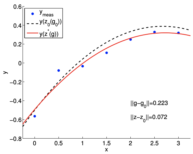
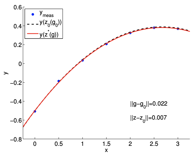
Example 17.3.4 Measurement Noise in Polynomial Fitting

Let us demonstrate the effect of perturbation in \(g\) - or the measurement error - in the context

(a) large perturbation

(b) small perturbation

Figure 17.6: The effect of data perturbation on the solution.

of polynomial fitting we considered earlier. As before, we assume that the output depends on the input quadratically according to \[y(x)=-\frac{1}{2}+\frac{2}{3} x-\frac{1}{8} c x^{2}\] with \(c=1\). We construct clean data \(g_{0} \in \mathbb{R}^{m}, m=7\), by evaluating \(y\) at \[x_{i}=(i-1) / 2, \quad i=1, \ldots, m\] and setting \[g_{0, i}=y\left(x_{i}\right), \quad i=1, \ldots, m\] Because \(g_{0}\) precisely follows the quadratic function, \(z_{0}=(-1 / 2,2 / 3,-1 / 8)\) satisfies the overdetermined system \(B z_{0}=g_{0}\). Recall that \(B\) is the \(m \times n\) Vandermonde matrix with the evaluation points \(\left\{x_{i}\right\}\).

We then construct perturbed data \(g\) by adding random noise to \(g_{0}\), i.e. \[g_{i}=g_{0, i}+\epsilon_{i}, \quad i=1, \ldots, m\] Then, we solve for the least-squares solution \(z^{*}\) of \(B z^{*}=g\).

The result of solving the polynomial fitting problem for two different perturbation levels is shown in Figure \(17.6\). For the large perturbation case, the perturbation in data and the error in the solution - both measured in 2-norm - are \[\left\|g-g_{0}\right\|=0.223 \text { and }\left\|z-z_{0}\right\|=0.072\] In contrast, the small perturbation case produces \[\left\|g-g_{0}\right\|=0.022 \text { and }\left\|z-z_{0}\right\|=0.007\] The results confirm that a smaller perturbation in data results in a smaller error in the solution. We can also verify the error bounds. The minimum singular value of the Vandermonde matrix is \[\nu_{\min }(B)=0.627 .\] Application of the (absolute) error bound to the large perturbation case yields \[0.072=\left\|z-z_{0}\right\| \leq \frac{1}{\nu_{\min }(B)}\left\|g-g_{0}\right\|=0.356 .\] The error bound is clearly satisfied. The error bound for the small perturbation case is similarly satisfied.

We now prove the error bounds.

Proof. To establish the absolute error bound, we first note that the solution to the clean problem, \(z_{0}\), and the solution to the perturbed problem, \(z^{*}\), satisfy the normal equation, i.e. \[B^{\mathrm{T}} B z_{0}=B^{\mathrm{T}} g_{0} \quad \text { and } \quad B^{\mathrm{T}} B z^{*}=B^{\mathrm{T}} g .\] Taking the difference of the two equations \[B^{\mathrm{T}} B\left(z^{*}-z_{0}\right)=B^{\mathrm{T}}\left(g-g_{0}\right) .\] Now, we multiply both sides by \(\left(z^{*}-z_{0}\right)^{\mathrm{T}}\) to obtain \[\begin{aligned} \text { (LHS }) &=\left(z^{*}-z_{0}\right)^{\mathrm{T}} B^{\mathrm{T}} B\left(z^{*}-z_{0}\right)=\left(B\left(z^{*}-z_{0}\right)\right)^{\mathrm{T}}\left(B\left(z^{*}-z_{0}\right)\right)=\left\|B\left(z^{*}-z_{0}\right)\right\|^{2} \\ \text { (RHS }) &=\left(z^{*}-z_{0}\right)^{\mathrm{T}} B^{\mathrm{T}}\left(g-g_{0}\right)=\left(B\left(z^{*}-z_{0}\right)\right)^{\mathrm{T}}\left(g-g_{0}\right) \leq\left\|B\left(z^{*}-z_{0}\right)\right\|\left\|g-g_{0}\right\|, \end{aligned}\] where we have invoked the Cauchy-Schwarz inequality on the right-hand side. Thus, we have \[\left\|B\left(z^{*}-z_{0}\right)\right\|^{2} \leq\left\|B\left(z^{*}-z_{0}\right)\right\|\left\|g-g_{0}\right\| \quad \Rightarrow \quad\left\|B\left(z^{*}-z_{0}\right)\right\| \leq\left\|g-g_{0}\right\| .\] We can bound the left-hand side from below using the definition of the minimum singular value \[\nu_{\min }(B)\left\|z^{*}-z_{0}\right\| \leq\left\|B\left(z^{*}-z_{0}\right)\right\| .\] Thus, we have \[\nu_{\min }\left\|z^{*}-z_{0}\right\| \leq\left\|B\left(z^{*}-z_{0}\right)\right\| \leq\left\|g-g_{0}\right\| \quad \Rightarrow \quad\left\|z^{*}-z_{0}\right\| \leq \frac{1}{\nu_{\min }(B)}\left\|g-g_{0}\right\|,\] which is the desired absolute error bound.

To obtain the relative error bound, we first divide the absolute error bound by \(\left\|z_{0}\right\|\) to obtain \[\frac{\left\|z^{*}-z_{0}\right\|}{\left\|z_{0}\right\|} \leq \frac{1}{\nu_{\min }(B)} \frac{\left\|g-g_{0}\right\|}{\left\|z_{0}\right\|}=\frac{1}{\nu_{\min }(B)} \frac{\left\|g-g_{0}\right\|}{\left\|g_{0}\right\|} \frac{\left\|g_{0}\right\|}{\left\|z_{0}\right\|} .\] To bound the quotient \(\left\|g_{0}\right\| /\left\|z_{0}\right\|\), we take the norm of both sides of \(B z_{0}=g_{0}\) and invoke the definition of the maximum singular value, i.e. \[\left\|g_{0}\right\|=\left\|B z_{0}\right\| \leq \nu_{\max }\left\|z_{0}\right\| \Rightarrow \frac{\left\|g_{0}\right\|}{\left\|z_{0}\right\|} \leq \nu_{\max } .\] Substituting the expression to the previous bound \[\frac{\left\|z^{*}-z_{0}\right\|}{\left\|z_{0}\right\|} \leq \frac{1}{\nu_{\min }(B)} \frac{\left\|g-g_{0}\right\|}{\left\|g_{0}\right\|} \frac{\left\|g_{0}\right\|}{\left\|z_{0}\right\|} \leq \frac{\nu_{\max }(B)}{\nu_{\min }(B)} \frac{\left\|g-g_{0}\right\|}{\left\|g_{0}\right\|},\] which is the desired relative error bound. Proof (using singular value decomposition). We start with the singular value decomposition of matrix \(B\), \[B=U \Sigma V^{\mathrm{T}}\] where \(U\) is an \(m \times m\) unitary matrix, \(V\) is an \(n \times n\) unitary matrix, and \(\Sigma\) is an \(m \times n\) diagonal matrix. In particular, \(\Sigma\) consists of singular values of \(B\) and is of the form \[\Sigma=\left(\begin{array}{cccc} \nu_{1} & & & \\ & \nu_{2} & & \\ & & \ddots & \\ & & & \nu_{n} \\ & & & \end{array}\right)=\left(\begin{array}{c} \widehat{\Sigma} \\ 0 \end{array}\right)\] The singular value decomposition exists for any matrix. The solution to the original problem is given by \[B z=g \quad \Rightarrow \quad U \Sigma V^{\mathrm{T}} z=g \quad \Rightarrow \quad \Sigma V^{\mathrm{T}} z=U^{\mathrm{T}} g .\] The solution to the least-squares problem is \[\begin{aligned} z^{*} &=\arg \min _{z}\|B z-g\|=\arg \min _{z}\left\|U \Sigma V^{\mathrm{T}} z-g\right\|=\arg \min _{z}\left\|\Sigma V^{\mathrm{T}} z-U^{\mathrm{T}} g\right\| \\ &=V\left(\arg \min _{\tilde{z}}\|\Sigma \tilde{z}-\tilde{g}\|\right), \end{aligned}\] where the third equality follows from the fact that the action by an unitary matrix does not alter the 2-norm, and we have made the substitutions \(\tilde{z}=V^{\mathrm{T}} z\) and \(\tilde{g}=U^{\mathrm{T}} g\). We note that because \(\Sigma\) is diagonal, the 2-norm to be minimized is particularly simple, \[\Sigma \tilde{z}-\tilde{g}=\Sigma=\left(\begin{array}{ccc} \nu_{1} & & \\ & \ddots & \\ & & \nu_{n} \\ & & \\ & & \end{array}\right)\left(\begin{array}{c} \tilde{z}_{1} \\ \vdots \\ \tilde{z}_{n} \end{array}\right)-\left(\begin{array}{c} \tilde{g}_{1} \\ \vdots \\ \tilde{g}_{n} \\ \tilde{g}_{n+1} \\ \vdots \\ \tilde{g}_{m} \end{array}\right) .\] Note that choosing \(\tilde{z}_{1}, \ldots, \tilde{z}_{n}\) only affects the first \(n\) component of the residual vector. Thus, we should pick \(\tilde{z}_{1}, \ldots, \tilde{z}_{n}\) such that \[\left(\begin{array}{ccc} \nu_{1} & & \\ & \ddots & \\ & & \nu_{n} \end{array}\right)\left(\begin{array}{c} \tilde{z}_{1} \\ \vdots \\ \tilde{z}_{n} \end{array}\right)=\left(\begin{array}{c} \tilde{g}_{1} \\ \vdots \\ \tilde{g}_{n} \end{array}\right) \Rightarrow \quad \tilde{z}_{i}=\frac{\tilde{g}_{i}}{\nu_{i}}, \quad i=1, \ldots, n .\] By introducing a \(n \times m\) restriction matrix that extracts the first \(n\) entries of \(\tilde{g}\), we can concisely write the above as \[\widehat{\Sigma} \tilde{z}=R \tilde{g} \quad \Rightarrow \quad \tilde{z}=\widehat{\Sigma}^{-1} R \tilde{g},\] and the solution to the least-squares problem as \[z^{*}=V \tilde{z}^{*}=V \widehat{\Sigma}^{-1} R \tilde{g}=V \widehat{\Sigma}^{-1} R U^{\mathrm{T}} g .\] The absolute condition number bound is obtained by \[\begin{aligned} \left\|z^{*}-z_{0}\right\| &=\left\|V \widehat{\Sigma}^{-1} R U^{\mathrm{T}}\left(g-g_{0}\right)\right\|=\frac{\left\|V \widehat{\Sigma}^{-1} R U^{\mathrm{T}}\left(g-g_{0}\right)\right\|}{\left\|g-g_{0}\right\|}\left\|g-g_{0}\right\| \\ & \leq\left(\sup _{\delta g} \frac{\left\|V \widehat{\Sigma}^{-1} R U^{\mathrm{T}} \delta g\right\|}{\|\delta g\|}\right)\left\|g-g_{0}\right\| . \end{aligned}\] The term in the parenthesis is bounded by noting that orthogonal transformations preserve the 2 -norm and that the restriction operator does not increase the 2-norm, i.e. \[\sup _{\delta g}\left(\frac{\left\|V \widehat{\Sigma}^{-1} R U^{\mathrm{T}} \delta g\right\|}{\|\delta g\|}\right)=\sup _{\delta \tilde{g}}\left(\frac{\left\|V \widehat{\Sigma}^{-1} R \delta \tilde{g}\right\|}{\|U \delta \tilde{g}\|}\right)=\sup _{\delta \tilde{g}}\left(\frac{\left\|\widehat{\Sigma}^{-1} R \delta \tilde{g}\right\|}{\|\delta \tilde{g}\|}\right) \leq \frac{1}{\nu_{\min }(B)} .\] Thus, we have the desired absolute error bound \[\left\|z^{*}-z_{0}\right\| \leq \frac{1}{\nu_{\min }(B)}\left\|g-g_{0}\right\| .\] Now let us consider the relative error bound. We first note that \[\frac{\left\|z^{*}-z_{0}\right\|}{\left\|z_{0}\right\|}=\frac{1}{\nu_{\min }(B)}\left\|g-g_{0}\right\| \frac{1}{\left\|z_{0}\right\|}=\frac{1}{\nu_{\min }(B)} \frac{\left\|g-g_{0}\right\|}{\left\|g_{0}\right\|} \frac{\left\|g_{0}\right\|}{\left\|z_{0}\right\|} .\] The term \(\left\|g_{0}\right\| /\left\|z_{0}\right\|\) can be bounded by expressing \(z_{0}\) in terms of \(g\) using the explicit expression for the least-squares solution, i.e. \[\frac{\left\|g_{0}\right\|}{\left\|z_{0}\right\|}=\frac{\left\|B z_{0}\right\|}{\left\|z_{0}\right\|}=\frac{\left\|U \Sigma V^{\mathrm{T}} z_{0}\right\|}{\left\|z_{0}\right\|} \leq \sup _{z} \frac{\left\|U \Sigma V^{\mathrm{T}} z\right\|}{\|z\|}=\sup _{\tilde{z}} \frac{\|U \Sigma \tilde{z}\|}{\|V \tilde{z}\|}=\sup _{\tilde{z}} \frac{\|\Sigma \tilde{z}\|}{\|\tilde{z}\|}=\nu_{\max }(B) .\] Thus, we have the relative error bound \[\frac{\left\|z^{*}-z_{0}\right\|}{\left\|z_{0}\right\|} \leq \frac{\nu_{\max }(B)}{\nu_{\min }(B)} \frac{\left\|g-g_{0}\right\|}{\left\|g_{0}\right\|} .\] This concludes the proof.

Error Bounds with Respect to Reduction in Space, \(B\)

Let us now consider a scenario that illustrates the effect of bias. Again, we start with an overdetermined linear system, \[B_{0} z_{0}=g,\] where \(B_{0} \in \mathbb{R}^{m \times n}\) with \(m>n\). We assume that \(z_{0}\) satisfies all \(m\) equations. We recall that, in the context of polynomial fitting, \(B_{0}\) is of the form, \[B_{0}=\left(\begin{array}{ccccc} 1 & x_{1} & x_{1}^{2} & \cdots & x_{1}^{n} \\ 1 & x_{2} & x_{2}^{2} & \cdots & x_{2}^{n} \\ \vdots & \vdots & \vdots & & \vdots \\ 1 & x_{m} & x_{m}^{2} & \cdots & x_{m}^{n} \end{array}\right),\] where \(m\) is the number of data points and \(n\) is the degree of polynomial. Now, suppose that we decide to use a \(p\)-th degree polynomial rather than the \(n\)-th degree polynomial, where \(p<n\). In other words, we can partition \(B_{0}\) into \[B_{0}=\left(B_{\mathrm{I}} \mid B_{\mathrm{II}}\right)=\left(\begin{array}{cccc|ccc} 1 & x_{1}^{1} & \cdots & x_{1}^{p} & x_{1}^{p+1} & \cdots & x_{1}^{n} \\ 1 & x_{2}^{1} & \cdots & x_{2}^{p} & x_{2}^{p+1} & \cdots & x_{m}^{n} \\ \vdots & \vdots & & \vdots & \vdots & & \vdots \\ 1 & x_{m}^{1} & \cdots & x_{m}^{p} & x_{m}^{p+1} & \cdots & x_{m}^{n} \end{array}\right)\] where \(B_{\mathrm{I}} \in \mathbb{R}^{m \times(p+1)}\) and \(B_{\mathrm{II}} \in \mathbb{R}^{m \times(n-p)}\). Then we can solve the least-squares problem resulting from the first partition, i.e. \[B_{\mathrm{I}} z^{*}=g .\] For convenience, let us also partition the solution to the original system \(z_{0}\) into two parts corresponding to \(B_{\mathrm{I}}\) and \(B_{\mathrm{II}}\), i.e. \[z_{0}=\left(\begin{array}{c} z_{\mathrm{I}} \\ z_{\mathrm{II}} \end{array}\right),\] where \(z_{\mathrm{I}} \in \mathbb{R}^{p+1}\) and \(z_{\mathrm{II}} \in \mathbb{R}^{n-p}\). The question is, how close are the coefficients \(z^{*}=\left(z_{1}, \ldots, z_{p-1}\right)\) of the reduced system compared to the coefficients of the first partition of the original system, \(z_{1}\) ?

We can in fact bound the error in the solution \(\left\|z^{*}-z_{\mathrm{I}}\right\|\) in terms of the "missing space" \(B_{\mathrm{II}}\). In particular, the absolute error bound is given by \[\left\|z^{*}-z_{\mathrm{I}}\right\| \leq \frac{1}{\nu_{\min }\left(B_{\mathrm{I}}\right)}\left\|B_{\mathrm{II}} z_{\mathrm{II}}\right\|\] and the relative error bound is given by \[\frac{\left\|z^{*}-z_{\mathrm{I}}\right\|}{\left\|z_{\mathrm{I}}\right\|} \leq \frac{\nu_{\max }\left(B_{\mathrm{I}}\right)}{\nu_{\min }\left(B_{\mathrm{I}}\right)} \frac{\left\|B_{\mathrm{II}} z_{\mathrm{II}}\right\|}{\left\|g-B_{\mathrm{II}} z_{\mathrm{II}}\right\|},\] where \(\nu_{\min }\left(B_{\mathrm{I}}\right)\) and \(\nu_{\max }\left(B_{\mathrm{I}}\right)\) are the minimum and maximum singular values of \(B_{\mathrm{I}}\).

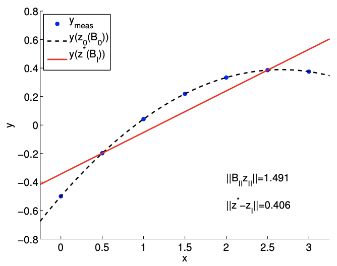
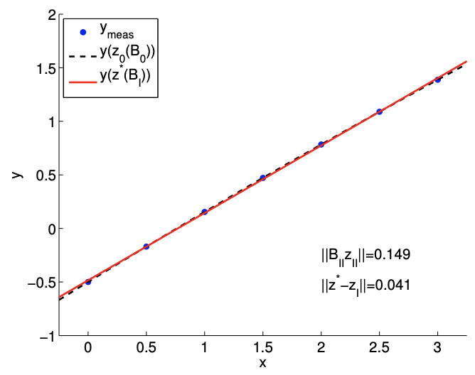
Example 17.3.5 Bias Effect in Polynomial Fitting

Let us demonstrate the effect of reduced solution space - or the bias effect - in the context of polynomial fitting. As before, the output depends on the input quadratically according to \[y(x)=-\frac{1}{2}+\frac{2}{3} x-\frac{1}{8} c x^{2} .\] Recall that \(c\) controls the strength of quadratic dependence. The data \(g\) is generated by evaluating \(y\) at \(x_{i}=(i-1) / 2\) and setting \(g_{i}=y\left(x_{i}\right)\) for \(i=1, \ldots, m\), with \(m=7\). We partition our Vandermonde matrix for the quadratic model \(B_{0}\) into that for the affine model \(B_{\mathrm{I}}\) and the quadratic only part \(B_{\mathrm{II}}\), i.e. \[B_{0}=\left(\begin{array}{ccc} 1 & x_{1} & x_{1}^{2} \\ 1 & x_{2} & x_{2}^{2} \\ \vdots & \vdots & \vdots \\ 1 & x_{m} & x_{m}^{2} \end{array}\right)=\left(\begin{array}{cc|c} 1 & x_{1} & x_{1}^{2} \\ 1 & x_{2} & x_{2}^{2} \\ \vdots & \vdots & \vdots \\ 1 & x_{m} & x_{m}^{2} \end{array}\right)=\left(B_{\mathrm{I}} \mid B_{\mathrm{II}}\right) .\]

(a) \(c=1\)

(b) \(c=1 / 10\)

Figure 17.7: The effect of reduction in space on the solution.

As before, because the underlying data is quadratic, we can exactly match the function using the full space \(B_{0}\), i.e., \(B_{0} z_{0}=g\).

Now, we restrict ourselves to affine functions, and find the least-squares solution \(z^{*}\) to \(B_{\mathrm{I}} z^{*}=g\). We would like to quantify the difference in the first two coefficients of the full model \(z_{I}\) and the coefficients of the reduced model \(z^{*}\).

Figure \(17.7\) shows the result of fitting an affine function to the quadratic function for \(c=1\) and \(c=1 / 10\). For the \(c=1\) case, with the strong quadratic dependence, the effect of the missing quadratic function is \[\left\|B_{\mathrm{II}} z_{\mathrm{II}}\right\|=1.491\] This results in a relative large solution error of \[\left\|z^{*}-z_{\mathrm{I}}\right\|=0.406\] We also note that, with the minimum singular value of \(\nu_{\min }\left(B_{\mathrm{I}}\right)=1.323\), the (absolute) error bound is satisfied as \[0.406=\left\|z^{*}-z_{\mathrm{I}}\right\| \leq \frac{1}{\nu_{\min }\left(B_{\mathrm{I}}\right)}\left\|B_{\mathrm{II}} z_{I I}\right\|=1.1267\] In fact, the bound in this particular case is reasonable sharp.

Recall that the least-squares solution \(z^{*}\) minimizes the \(\ell_{2}\) residual \[0.286=\left\|B_{\mathrm{I}} z^{*}-g\right\| \leq\left\|B_{\mathrm{I}} z-g\right\|, \quad \forall z \in \mathbb{R}^{2}\] and the residual is in particular smaller than that for the truncated solution \[\left\|B_{\mathrm{I}} z_{\mathrm{I}}-g\right\|=1.491\] However, the error for the least-squares solution - in terms of predicting the first two coefficients of the underlying polynomial - is larger than that of the truncated solution (which of course is zero). This case demonstrates that minimizing the residual does not necessarily minimize the error. For the \(c=1 / 10\) with a weaker quadratic dependence, the effect of missing the quadratic function is \[\left\|B_{\mathrm{II}} z_{\mathrm{II}}\right\|=0.149\] and the error in the solution is accordingly smaller as \[\left\|z^{*}-z_{\mathrm{I}}\right\|=0.041 .\] This agrees with our intuition. If the underlying data exhibits a weak quadratic dependence, then we can represent the data well using an affine function, i.e., \(\left\|B_{\mathrm{II}} z_{\mathrm{II}}\right\|\) is small. Then, the (absolute) error bound suggests that the small residual results in a small error.

We now prove the error bound.

Proof. We rearrange the original system as \[B_{0} z_{0}=B_{\mathrm{I}} z_{\mathrm{I}}+B_{\mathrm{II}} z_{\mathrm{II}}=g \quad \Rightarrow \quad B_{\mathrm{I}} z_{\mathrm{I}}=g-B_{\mathrm{II}} z_{\mathrm{II}} .\] By our assumption, there is a solution \(z_{\mathrm{I}}\) that satisfies the \(m \times(p+1)\) overdetermined system \[B_{\mathrm{I}} z_{\mathrm{I}}=g-B_{\mathrm{II}} z_{\mathrm{II}} .\] The reduced system, \[B_{\mathrm{I}} z^{*}=g,\] does not have a solution in general, so is solved in the least-squares sense. These two cases are identical to the unperturbed and perturbed right-hand side cases considered the previous subsection. In particular, the perturbation in the right-hand side is \[\left\|g-\left(g-B_{\mathrm{II}} z_{\mathrm{II}}\right)\right\|=\left\|B_{\mathrm{II}} z_{\mathrm{II}}\right\|,\] and the perturbation in the solution is \(\left\|z^{*}-z_{\mathrm{I}}\right\|\). Substitution of the perturbations into the absolute and relative error bounds established in the previous subsection yields the desired results.

Advanced Material