19.1: Simplest Case

Let us first consider a "simple" case of regression, where we restrict ourselves to one independent variable and linear basis functions.

Friction Coefficient Determination Problem Revisited

Recall the friction coefficient determination problem we considered in Section \(17.1\). We have seen that in presence of \(m\) perfect measurements, we can find a \(\mu_{\mathrm{s}}\) that satisfies \(m\) equations \[F_{\mathrm{f}, \text { static } i}^{\max }=\mu_{\mathrm{s}} F_{\text {normal, applied } i}, \quad i=1, \ldots, m\] In other words, we can use any one of the \(m\)-measurements and solve for \(\mu_{s}\) according to \[\mu_{\mathrm{s}, i}=\frac{F_{\mathrm{f}, \text { static } i}^{\max , \text { meas }}}{F_{\text {normal, applied } i}}\] and all \(\mu_{\mathrm{s}, i}, i=1, \ldots, m\), will be identical and agree with the true value \(\mu_{\mathrm{s}}\).

Unfortunately, real measurements are corrupted by noise. In particular, it is unlikely that we can find a single coefficient that satisfies all \(m\) measurement pairs. In other words, \(\mu_{\mathrm{s}}\) computed using the \(m\) different pairs are likely not to be identical. A more suitable model for static friction that incorporates the notion of measurement noise is \[F_{\mathrm{f}, \text { static }}^{\max , \text { meas }}=\mu_{\mathrm{S}} F_{\text {normal, applied }}+\epsilon .\] The noise associated with each measurement is obviously unknown (otherwise we could correct the measurements), so the equation in the current form is not very useful. However, if we make some weak assumptions on the behavior of the noise, we can in fact:

(a) infer the value of \(\mu_{\mathrm{s}}\) with associated confidence,

(b) estimate the noise level,

(c) confirm that our model is correct (more precisely, not incorrect),

(d) and detect significant unmodeled effects. This is the idea behind regression — a framework for deducing the relationship between a set of inputs (e.g. \(F_{\text {normal,applied }}\) ) and the outputs (e.g. \(F_{\mathrm{f}, \text { static }}^{\text {max }}\) ) in the presence of noise. The regression framework consists of two steps: \((i)\) construction of an appropriate response model, and (ii) identification of the model parameters based on data. We will now develop procedures for carrying out these tasks.

Response Model

Let us describe the relationship between the input \(x\) and output \(Y\) by \[Y(x)=Y_{\text {model }}(x ; \beta)+\epsilon(x),\] where

(a) \(x\) is the independent variable, which is deterministic.

(b) \(Y\) is the measured quantity (i.e., data), which in general is noisy. Because the noise is assumed to be random, \(Y\) is a random variable.

(c) \(Y_{\text {model }}\) is the predictive model with no noise. In linear regression, \(Y_{\text {model }}\) is a linear function of the model parameter \(\beta\) by definition. In addition, we assume here that the model is an affine function of \(x\), i.e. \[Y_{\text {model }}(x ; \beta)=\beta_{0}+\beta_{1} x,\] where \(\beta_{0}\) and \(\beta_{1}\) are the components of the model parameter \(\beta\). We will relax this affine-in- \(x\) assumption in the next section and consider more general functional dependencies as well as additional independent variables.

\((d) \epsilon\) is the noise, which is a random variable.

Our objective is to infer the model parameter \(\beta\) that best describes the behavior of the measured quantity and to build a model \(Y_{\text {model }}(\cdot ; \beta)\) that can be used to predict the output for a new \(x\). (Note that in some cases, the estimation of the parameter itself may be of interest, e.g. deducing the friction coefficient. In other cases, the primary interest may be to predict the output using the model, e.g. predicting the frictional force for a given normal force. In the second case, the parameter estimation itself is simply a means to the end.)

As considered in Section 17.1, we assume that our model is unbiased. That is, in the absence of noise \((\epsilon=0)\), our underlying input-output relationship can be perfectly described by \[y(x)=Y_{\text {model }}\left(x ; \beta^{\text {true }}\right)\] for some "true" parameter \(\beta^{\text {true }}\). In other words, our model includes the true functional dependency (but may include more generality than is actually needed). We observed in Section \(17.1\) that if the model is unbiased and measurements are noise-free, then we can deduce the true parameter, \(\beta^{\text {true }}\), using a number of data points equal to or greater than the degrees of freedom of the model \((m \geq n)\).

In this chapter, while we still assume that the model is unbiased \({ }_{-}^{1}\), we relax the noise-free assumption. Our measurement (i.e., data) is now of the form \[Y(x)=Y_{\text {model }}\left(x ; \beta^{\text {true }}\right)+\epsilon(x),\] where \(\epsilon\) is the noise. In order to estimate the true parameter, \(\beta^{\text {true }}\), with confidence, we make three important assumptions about the behavior of the noise. These assumptions allow us to make quantitative (statistical) claims about the quality of our regression.

\({ }^{1}\) In Section 19.2.4, we will consider effects of bias (or undermodelling) in one of the examples.

Figure 19.1: Illustration of the regression process.

(\(i\)) Normality (N1): We assume the noise is a normally distributed with zero-mean, i.e., \(\epsilon(x) \sim\) \(\mathcal{N}\left(0, \sigma^{2}(x)\right)\). Thus, the noise \(\epsilon(x)\) is described by a single parameter \(\sigma^{2}(x)\).

(\(ii\)) Homoscedasticity (N2): We assume that \(\epsilon\) is not a function of \(x\) in the sense that the distribution of \(\epsilon\), in particular \(\sigma^{2}\), does not depend on \(x\).

(\(iii\)) Independence (N3): We assume that \(\epsilon\left(x_{1}\right)\) and \(\epsilon\left(x_{2}\right)\) are independent and hence uncorrelated.

We will refer to these three assumptions as (N1), (N2), and (N3) throughout the rest of the chapter. These assumptions imply that \(\epsilon(x)=\epsilon=\mathcal{N}\left(0, \sigma^{2}\right)\), where \(\sigma^{2}\) is the single parameter for all instances of \(x\).

Note that because \[Y(x)=Y_{\text {model }}(x ; \beta)+\epsilon=\beta_{0}+\beta_{1} x+\epsilon\] and \(\epsilon \sim \mathcal{N}\left(0, \sigma^{2}\right)\), the deterministic model \(Y_{\text {model }}(x ; \beta)\) simply shifts the mean of the normal distribution. Thus, the measurement is a random variable with the distribution \[Y(x) \sim \mathcal{N}\left(Y_{\text {model }}(x ; \beta), \sigma^{2}\right)=\mathcal{N}\left(\beta_{0}+\beta_{1} x, \sigma^{2}\right) .\] In other words, when we perform a measurement at some point \(x_{i}\), we are in theory drawing a random variable from the distribution \(\mathcal{N}\left(\beta_{0}+\beta_{1} x_{i}, \sigma^{2}\right)\). We may think of \(Y(x)\) as a random variable (with mean) parameterized by \(x\), or we may think of \(Y(x)\) as a random function (often denoted a random process).

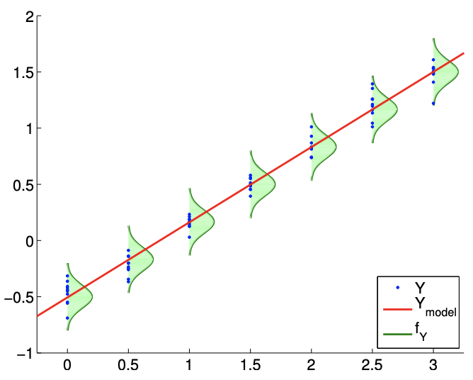
A typical regression process is illustrated in Figure 19.1. The model \(Y_{\text {model }}\) is a linear function of the form \(\beta_{0}+\beta_{1} x\). The probability density functions of \(Y, f_{Y}\), shows that the error is normally distributed (N1) and that the variance does not change with \(x\) (N2). The realizations of \(Y\) sampled for \(x=0.0,0.5,1.0, \ldots, 3.0\) confirms that it is unlikely for realizations to fall outside of the \(3 \sigma\) bounds plotted. (Recall that \(99.7 \%\) of the samples falls within the \(3 \sigma\) bounds for a normal distribution.)

Figure \(19.1\) suggests that the likely outcome of \(Y\) depends on our independent variable \(x\) in a linear manner. This does not mean that \(Y\) is a function of \(x\) only. In particular, the outcome of an experiment is in general a function of many independent variables, \[x=\left(\begin{array}{llll} x_{(1)} & x_{(2)} & \cdots & x_{(k)} \end{array}\right)\] But, in constructing our model, we assume that the outcome only strongly depends on the behavior of \(x=x_{(1)}\), and the net effect of the other variables \(\left(\begin{array}{ccc}x_{(2)} & \cdots & x_{(k)}\end{array}\right)\) can be modeled as random through \(\epsilon\). In other words, the underlying process that governs the input-output relationship may be completely deterministic if we are given \(k\) variables that provides the full description of the system, i.e. \[y\left(x_{(1)}, x_{(2)}, \ldots, x_{(k)}\right)=f\left(x_{(1)}, x_{(2)}, \ldots, x_{(k)}\right) .\] However, it is unlikely that we have the full knowledge of functional dependencies as well as the state of the system.

Knowing that the deterministic prediction of the output is intractable, we resort to understanding the functional dependency of the most significant variable, say \(x_{(1)}\). If we know that the dependency of \(y\) on \(x_{(1)}\) is most dominantly affine (say based on a physical law), then we can split our (intractable) functional dependency into \[y\left(x_{(1)}, x_{(2)}, \ldots, x_{(k)}\right)=\beta_{0}+\beta_{1} x_{(1)}+g\left(x_{(1)}, x_{(2)}, \ldots, x_{(k)}\right) .\] Here \(g\left(x_{(1)}, x_{(2)}, \ldots, x_{(k)}\right)\) includes both the unmodeled system behavior and the unmodeled process that leads to measurement errors. At this point, we assume the effect of \(\left(x_{(2)}, \ldots, x_{(k)}\right)\) on \(y\) and the weak effect of \(x_{(1)}\) on \(y\) through \(g\) can be lumped into a zero-mean random variable \(\epsilon\), i.e. \[Y\left(x_{(1)} ; \beta\right)=\beta_{0}+\beta_{1} x_{(1)}+\epsilon .\] At some level this equation is almost guaranteed to be wrong.

First, there will be some bias: here bias refers to a deviation of the mean of \(Y(x)\) from \(\beta_{0}+\beta_{1} x_{(1)}\) - which of course can not be represented by \(\epsilon\) which is assumed zero mean. Second, our model for the noise (e.g., (N1), (N2), (N3)) - indeed, any model for noise - is certainly not perfect. However, if the bias is small, and the deviations of the noise from our assumptions (N1), (N2), and (N3) are small, our procedures typically provide good answers. Hence we must always question whether the response model \(Y_{\text {model }}\) is correct, in the sense that it includes the correct model. Furthermore, the assumptions (N1), (N2), and (N3) do not apply to all physical processes and should be treated with skepticism.

We also note that the appropriate number of independent variables that are explicitly modeled, without being lumped into the random variable, depends on the system. (In the next section, we will treat the case in which we must consider the functional dependencies on more than one independent variable.) Let us solidify the idea using a very simple example of multiple coin flips in which in fact we need not consider any independent variables.

Example 19.1.1 Functional dependencies in coin flips

Let us say the system is 100 fair coin flips and \(Y\) is the total number of heads. The outcome of each coin flip, which affects the output \(Y\), is a function of many variables: the mass of the coin, the moment of inertia of the coin, initial launch velocity, initial angular momentum, elasticity of the surface, density of the air, etc. If we had a complete description of the environment, then the outcome of each coin flip is deterministic, governed by Euler’s equations (for rigid body dynamics), the Navier-Stokes equations (for air dynamics), etc. We see this deterministic approach renders our simulation intractable - both in terms of the number of states and the functional dependencies even for something as simple as coin flips.

Thus, we take an alternative approach and lump some of the functional dependencies into a random variable. From Chapter 9 , we know that \(Y\) will have a binomial distribution \(\mathcal{B}(n=100, \theta=\) \(1 / 2)\). The mean and the variance of \(Y\) are \[E[Y]=n \theta=50 \text { and } E\left[\left(Y-\mu_{Y}\right)^{2}\right]=n \theta(1-\theta)=25 .\] In fact, by the central limit theorem, we know that \(Y\) can be approximated by \[Y \sim \mathcal{N}(50,25) .\] The fact that \(Y\) can be modeled as \(\mathcal{N}(50,25)\) without any explicit dependence on any of the many independent variables we cited earlier does not mean that \(Y\) does not depend on the variables. It only means that the cumulative effect of the all independent variables on \(Y\) can be modeled as a zero-mean normal random variable. This can perhaps be motivated more generally by the central limit theorem, which heuristically justifies the treatment of many small random effects as normal noise.

Parameter Estimation

We now perform \(m\) experiments, each of which is characterized by the independent variable \(x_{i}\). Each experiment described by \(x_{i}\) results in a measurement \(Y_{i}\), and we collect \(m\) variable-measurement pairs, \[\left(x_{i}, Y_{i}\right), \quad i=1, \ldots, m .\] In general, the value of the independent variables \(x_{i}\) can be repeated. We assume that our measurements satisfy \[Y_{i}=Y_{\text {model }}\left(x_{i} ; \beta\right)+\epsilon_{i}=\beta_{0}+\beta_{1} x_{i}+\epsilon_{i} .\] From the experiments, we wish to estimate the true parameter \(\beta^{\text {true }}=\left(\beta_{0}^{\text {true }}, \beta_{1}^{\text {true }}\right)\) without the precise knowledge of \(\epsilon\) (which is described by \(\sigma\) ). In fact we will estimate \(\beta^{\text {true }}\) and \(\sigma\) by \(\hat{\beta}\) and \(\hat{\sigma}\), respectively.

It turns out, from our assumptions (N1), (N2), and (N3), that the maximum likelihood estimator (MLE) for \(\beta\) - the most likely value for the parameter given the measurements \(\left(x_{i}, Y_{i}\right), i=1, \ldots, m\) - is precisely our least squares fit, i.e., \(\hat{\beta}=\beta^{*}\). In other words, if we form \[X=\left(\begin{array}{cc} 1 & x_{1} \\ 1 & x_{2} \\ \vdots & \vdots \\ 1 & x_{m} \end{array}\right) \quad \text { and } \quad Y=\left(\begin{array}{c} Y_{1} \\ Y_{2} \\ \vdots \\ Y_{m} \end{array}\right)\] then the MLE, \(\hat{\beta}\), satisfies \[\|X \hat{\beta}-Y\|_{2}<\|X \beta-Y\|_{2}, \quad \forall \beta \neq \hat{\beta} .\] Equivalently, \(\hat{\beta}\) satisfies the normal equation \[\left(X^{\mathrm{T}} X\right) \hat{\beta}=X^{\mathrm{T}} Y .\] We provide the proof.

Proof

We show that the least squares solution is the maximum likelihood estimator (MLE) for \(\beta\). Recall that we consider each measurement as \(Y_{i}=\mathcal{N}\left(\beta_{0}+\beta_{1} x_{i}, \sigma^{2}\right)=\mathcal{N}\left(X_{i} \cdot \beta, \sigma^{2}\right)\). Noting the noise is independent, the \(m\) measurement collectively defines a joint distribution, \[Y=\mathcal{N}(X \beta, \Sigma),\] where \(\Sigma\) is the diagonal covariance matrix \(\Sigma=\operatorname{diag}\left(\sigma^{2}, \ldots, \sigma^{2}\right)\). To find the MLE, we first form the conditional probability density of \(Y\) assuming \(\beta\) is given, i.e. \[f_{Y \mid \mathcal{B}}(y \mid \beta)=\frac{1}{(2 \pi)^{m / 1}|\Sigma|^{1 / 2}} \exp \left(-\frac{1}{2}(y-X \beta)^{\mathrm{T}} \Sigma^{-1}(y-X \beta)\right),\] which can be viewed as a likelihood function if we now fix \(y\) and let \(\beta\) vary \(-\beta \mid y\) rather than \(y \mid \beta\). The MLE - the \(\beta\) that maximizes the likelihood of measurements \(\left\{y_{i}\right\}_{i=1}^{m}\) - is then \[\hat{\beta}=\arg \max _{\beta \in \mathbb{R}^{2}} f_{Y \mid \mathcal{B}}(y \mid \beta)=\arg \max _{\beta \in \mathbb{R}^{2}} \frac{1}{(2 \pi)^{m / 1}|\Sigma|^{1 / 2}} \exp (-\underbrace{\frac{1}{2}(y-X \beta)^{\mathrm{T}} \Sigma^{-1}(y-X \beta)}_{J}) .\] The maximum is obtained when \(J\) is minimized. Thus, \[\hat{\beta}=\arg \min _{\beta \in \mathbb{R}^{2}} J(\beta)=\arg \min _{\beta \in \mathbb{R}^{2}} \frac{1}{2}(y-X \beta)^{\mathrm{T}} \Sigma^{-1}(y-X \beta) .\] Recalling the form of \(\Sigma\), we can simplify the expression to \[\begin{aligned} \hat{\beta} &=\arg \min _{\beta \in \mathbb{R}^{2}} \frac{1}{2 \sigma^{2}}(y-X \beta)^{\mathrm{T}}(y-X \beta)=\arg \min _{\beta \in \mathbb{R}^{2}}(y-X \beta)^{\mathrm{T}}(y-X \beta) \\ &=\arg \min _{\beta \in \mathbb{R}^{2}}\|y-X \beta\|^{2} . \end{aligned}\] This is precisely the least squares problem. Thus, the solution to the least squares problem \(X \beta=y\) is the MLE.

Having estimated the unknown parameter \(\beta^{\text {true }}\) by \(\hat{\beta}\), let us now estimate the noise \(\epsilon\) characterized by the unknown \(\sigma\) (which we may think of as \(\sigma^{\text {true }}\) ). Our estimator for \(\sigma, \hat{\sigma}\), is \[\hat{\sigma}=\left(\frac{1}{m-2}\|Y-X \hat{\beta}\|^{2}\right)^{1 / 2} .\] Note that \(\|Y-X \hat{\beta}\|\) is just the root mean square of the residual as motivated by the least squares approach earlier. The normalization factor, \(1 /(m-2)\), comes from the fact that there are \(m\) measurement points and two parameters to be fit. If \(m=2\), then all the data goes to fitting the parameters \(\left\{\beta_{0}, \beta_{1}\right\}\) - two points determine a line - and none is left over to estimate the error; thus, in this case, we cannot estimate the error. Note that \[(X \hat{\beta})_{i}=\left.Y_{\text {model }}\left(x_{i} ; \beta\right)\right|_{\beta=\hat{\beta}} \equiv \widehat{Y}_{i}\] is our response model evaluated at the parameter \(\beta=\hat{\beta}\); we may thus write \[\hat{\sigma}=\left(\frac{1}{m-2}\|Y-\widehat{Y}\|^{2}\right)^{1 / 2} .\] In some sense, \(\hat{\beta}\) minimizes the misfit and what is left is attributed to noise \(\hat{\sigma}\) (per our model). Note that we use the data at all points, \(x_{1}, \ldots, x_{m}\), to obtain an estimate of our single parameter, \(\sigma\); this is due to our homoscedasticity assumption (N2), which assumes that \(\epsilon\) (and hence \(\sigma\) ) is independent of \(x\).

We also note that the least squares estimate preserves the mean of the measurements in the sense that \[\bar{Y} \equiv \frac{1}{m} \sum_{i=1}^{m} Y_{i}=\frac{1}{m} \sum_{i=1}^{m} \widehat{Y}_{i} \equiv \overline{\widehat{Y}}\]

Proof

The preservation of the mean is a direct consequence of the estimator \(\hat{\beta}\) satisfying the normal equation. Recall, \(\hat{\beta}\) satisfies \[X^{\mathrm{T}} X \hat{\beta}=X^{\mathrm{T}} Y .\] Because \(\widehat{Y}=X \hat{\beta}\), we can write this as \[X^{\mathrm{T}} \widehat{Y}=X^{\mathrm{T}} Y\] Recalling the "row" interpretation of matrix-vector product and noting that the column of \(X\) is all ones, the first component of the left-hand side is \[\left(X^{\mathrm{T}} \widehat{Y}\right)_{1}=\left(\begin{array}{lll} 1 & \cdots & 1 \end{array}\right)\left(\begin{array}{c} \widehat{Y}_{1} \\ \vdots \\ \widehat{Y}_{m} \end{array}\right)=\sum_{i=1}^{m} \widehat{Y}_{i}\] Similarly, the first component of the right-hand side is \[\left(X^{\mathrm{T}} Y\right)_{1}=\left(\begin{array}{lll} 1 & \cdots & 1 \end{array}\right)\left(\begin{array}{c} Y_{1} \\ \vdots \\ Y_{m} \end{array}\right)=\sum_{i=1}^{m} Y_{i}\] Thus, we have \[\left(X^{\mathrm{T}} \widehat{Y}\right)_{1}=\left(X^{\mathrm{T}} Y\right)_{1} \quad \Rightarrow \quad \sum_{i=1}^{m} \widehat{Y}_{i}=\sum_{i=1}^{m} Y_{i},\] which proves that the model preserves the mean.

Confidence Intervals

We consider two sets of confidence intervals. The first set of confidence intervals, which we refer to as individual confidence intervals, are the intervals associated with each individual parameter. The second set of confidence intervals, which we refer to as joint confidence intervals, are the intervals associated with the joint behavior of the parameters.

Individual Confidence Intervals

Let us introduce an estimate for the covariance of \(\hat{\beta}\), \[\widehat{\Sigma} \equiv \hat{\sigma}^{2}\left(X^{\mathrm{T}} X\right)^{-1} .\] For our case with two parameters, the covariance matrix is \(2 \times 2\). From our estimate of the covariance, we can construct the confidence interval for \(\beta_{0}\) as \[I_{0} \equiv\left[\hat{\beta}_{0}-t_{\gamma, m-2} \sqrt{\widehat{\Sigma}_{11}}, \hat{\beta}_{0}+t_{\gamma, m-2} \sqrt{\widehat{\Sigma}_{11}}\right],\] and the confidence interval for \(\beta_{1}\) as \[I_{1} \equiv\left[\hat{\beta}_{1}-t_{\gamma, m-2} \sqrt{\widehat{\Sigma}_{22}}, \hat{\beta}_{1}+t_{\gamma, m-2} \sqrt{\widehat{\Sigma}_{22}}\right] .\] The coefficient \(t_{\gamma, m-2}\) depends on the confidence level, \(\gamma\), and the degrees of freedom, \(m-2\). Note that the Half Length of the confidence intervals for \(\beta_{0}\) and \(\beta_{1}\) are equal to \(t_{\gamma, m-2} \sqrt{\widehat{\Sigma}_{11}}\) and \(t_{\gamma, m-2} \sqrt{\widehat{\Sigma}_{22}}\), respectively.

The confidence interval \(I_{0}\) is an interval such that the probability of the parameter \(\beta_{0}^{\text {true }}\) taking on a value within the interval is equal to the confidence level \(\gamma\), i.e. \[P\left(\beta_{0}^{\text {true }} \in I_{0}\right)=\gamma .\] Separately, the confidence interval \(I_{1}\) satisfies \[P\left(\beta_{1}^{\text {true }} \in I_{1}\right)=\gamma .\] The parameter \(t_{\gamma, q}\) is the value that satisfies \[\int_{-t_{\gamma, q}}^{t_{\gamma, q}} f_{T, q}(s) d s=\gamma,\] where \(f_{T, q}\) is the probability density function for the Student’s \(t\)-distribution with \(q\) degrees of freedom. We recall the frequentistic interpretation of confidence intervals from our earlier estmation discussion of Unit II.

Note that we can relate \(t_{\gamma, q}\) to the cumulative distribution function of the \(t\)-distribution, \(F_{T, q}\), as follows. First, we note that \(f_{T, q}\) is symmetric about zero. Thus, we have \[\int_{0}^{t_{\gamma, q}} f_{T, q}(s) d s=\frac{\gamma}{2}\] and \[F_{T, q}(x) \equiv \int_{-\infty}^{x} f_{T, q}(s) d s=\frac{1}{2}+\int_{0}^{x} f_{T, q}(s) d s .\] Evaluating the cumulative distribution function at \(t_{\gamma, q}\) and substituting the desired integral relationship, \[F_{T, q}\left(t_{\gamma, q}\right)=\frac{1}{2}+\int_{0}^{t_{\gamma, q}} f_{T, q}\left(t_{\gamma, q}\right) d s=\frac{1}{2}+\frac{\gamma}{2} .\] In particular, given an inverse cumulative distribution function for the Student’s \(t\)-distribution, we can readily compute \(t_{\gamma, q}\) as \[t_{\gamma, q}=F_{T, q}^{-1}\left(\frac{1}{2}+\frac{\gamma}{2}\right) .\] For convenience, we have tabulated the coefficients for \(95 \%\) confidence level for select values of degrees of freedom in Table 19.1(a).

\(q\)	\(t_{\gamma, q} \mid \gamma=0.95\)
10	\(2.228\)
15	\(2.131\)
20	\(2.086\)
25	\(2.060\)
30	\(2.042\)
40	\(2.021\)
5	\(2.571\)
50	\(2.009\)
60	\(2.000\)
\(\infty\)	\(1.960\)

(a) \(t\)-distribution

\(q\)	\(k=1\)	2	3	4	5	10	15	20
5	\(2.571\)	\(3.402\)	\(4.028\)	\(4.557\)	\(5.025\)	\(6.881\)	\(8.324\)	\(9.548\)
10	\(2.228\)	\(2.865\)	\(3.335\)	\(3.730\)	\(4.078\)	\(5.457\)	\(6.533\)	\(7.449\)
15	\(2.131\)	\(2.714\)	\(3.140\)	\(3.496\)	\(3.809\)	\(5.044\)	\(6.004\)	\(6.823\)
20	\(2.086\)	\(2.643\)	\(3.049\)	\(3.386\)	\(3.682\)	\(4.845\)	\(5.749\)	\(6.518\)
25	\(2.060\)	\(2.602\)	\(2.996\)	\(3.322\)	\(3.608\)	\(4.729\)	\(5.598\)	\(6.336\)
30	\(2.042\)	\(2.575\)	\(2.961\)	\(3.280\)	\(3.559\)	\(4.653\)	\(5.497\)	\(6.216\)
40	\(2.021\)	\(2.542\)	\(2.918\)	\(3.229\)	\(3.500\)	\(4.558\)	\(5.373\)	\(6.064\)
50	\(2.009\)	\(2.523\)	\(2.893\)	\(3.198\)	\(3.464\)	\(4.501\)	\(5.298\)	\(5.973\)
60	\(2.000\)	\(2.510\)	\(2.876\)	\(3.178\)	\(3.441\)	\(4.464\)	\(5.248\)	\(5.913\)
\(\infty\)	\(1.960\)	\(2.448\)	\(2.796\)	\(3.080\)	\(3.327\)	\(4.279\)	\(5.000\)	\(5.605\)

(b) \(F\)-distribution

Table 19.1: The coefficient for computing the \(95 \%\) confidence interval from Student’s \(t\)-distribution and \(F\)-distribution.

Joint Confidence Intervals

Sometimes we are more interested in constructing joint confidence intervals - confidence intervals within which the true values of all the parameters lie in a fraction \(\gamma\) of all realizations. These confidence intervals are constructed in essentially the same manner as the individual confidence intervals and take on a similar form. Joint confidence intervals for \(\beta_{0}\) and \(\beta_{1}\) are of the form \[I_{0}^{\text {joint }} \equiv\left[\hat{\beta}_{0}-s_{\gamma, 2, m-2} \sqrt{\widehat{\Sigma}_{11}}, \hat{\beta}_{0}+s_{\gamma, 2, m-2} \sqrt{\widehat{\Sigma}_{11}}\right]\] and \[I_{1}^{\text {joint }} \equiv\left[\hat{\beta}_{1}-s_{\gamma, 2, m-2} \sqrt{\widehat{\Sigma}_{22}}, \hat{\beta}_{1}+s_{\gamma, 2, m-2} \sqrt{\widehat{\Sigma}_{22}}\right]\] Note that the parameter \(t_{\gamma, m-2}\) has been replaced by a parameter \(s_{\gamma, 2, m-2}\). More generally, the parameter takes the form \(s_{\gamma, n, m-n}\), where \(\gamma\) is the confidence level, \(n\) is the number of parameters in the model (here \(n=2\) ), and \(m\) is the number of measurements. With the joint confidence interval, we have \[P\left(\beta_{0}^{\text {true }} \in I_{0}^{\text {joint }} \text { and } \beta_{1}^{\text {true }} \in I_{1}^{\text {joint }}\right) \geq \gamma\] Note the inequality - \(\geq \gamma-\) is because our intervals are a "bounding box" for the actual sharp confidence ellipse.

The parameter \(s_{\gamma, k, q}\) is related to \(\gamma\)-quantile for the \(F\)-distribution, \(g_{\gamma, k, q}\), by \[s_{\gamma, k, q}=\sqrt{k g_{\gamma, k, q}}\] Note \(g_{\gamma, k, q}\) satisfies \[\int_{0}^{g_{\gamma, k, q}} f_{F, k, q}(s) d s=\gamma\] where \(f_{F, k, q}\) is the probability density function of the \(F\)-distribution; we may also express \(g_{\gamma, k, q}\) in terms of the cumulative distribution function of the \(F\)-distribution as \[F_{F, k, q}\left(g_{\gamma, k, q}\right)=\int_{0}^{g_{\gamma, k, q}} f_{F, k, q}(s) d s=\gamma\] In particular, we can explicitly write \(s_{\gamma, k, q}\) using the inverse cumulative distribution for the \(F\) distribution, i.e. \[s_{\gamma, k, q}=\sqrt{k g_{\gamma, k, q}}=\sqrt{k F_{F, k, q}^{-1}(\gamma)} .\] For convenience, we have tabulated the values of \(s_{\gamma, k, q}\) for several different combinations of \(k\) and \(q\) in Table 19.1(b).

We note that \[s_{\gamma, k, q}=t_{\gamma, q}, \quad k=1,\] as expected, because the joint distribution is same as the individual distribution for the case with one parameter. Furthermore, \[s_{\gamma, k, q}>t_{\gamma, q}, \quad k>1,\] indicating that the joint confidence intervals are larger than the individual confidence intervals. In other words, the individual confidence intervals are too small to yield jointly the desired \(\gamma\).

We can understand these confidence intervals with some simple examples.

Example 19.1.2 least-squares estimate for a constant model

Let us consider a simple response model of the form \[Y_{\text {model }}(x ; \beta)=\beta_{0},\] where \(\beta_{0}\) is the single parameter to be determined. The overdetermined system is given by \[\left(\begin{array}{c} Y_{1} \\ Y_{2} \\ \vdots \\ Y_{m} \end{array}\right)=\left(\begin{array}{c} 1 \\ 1 \\ \vdots \\ 1 \end{array}\right) \beta_{0}=X \beta_{0}\] and we recognize \(X=\left(\begin{array}{llll}1 & 1 & \cdots & 1\end{array}\right)^{\mathrm{T}}\). Note that we have \[X^{\mathrm{T}} X=m\] For this simple system, we can develop an explicit expression for the least squares estimate for \(\beta_{0}^{\text {true }}, \hat{\beta}_{0}\) by solving the normal equation, i.e. \[X^{\mathrm{T}} X \hat{\beta}_{0}=X^{\mathrm{T}} Y \quad \Rightarrow \quad m \hat{\beta}_{0}=\sum_{i=1}^{m} Y_{i} \quad \Rightarrow \quad \hat{\beta}_{0}=\frac{1}{m} \sum_{i=1}^{m} Y_{i}\] Our parameter estimator \(\hat{\beta}_{0}\) is (not surprisingly) identical to the sample mean of Chapter 11 since our model here \(Y=\mathcal{N}\left(\beta_{0}^{\text {true }}, \sigma^{2}\right)\) is identical to the model of Chapter 11 .

The covariance matrix (which is a scalar for this case), \[\widehat{\Sigma}=\hat{\sigma}^{2}\left(X^{\mathrm{T}} X\right)^{-1}=\hat{\sigma}^{2} / m .\] Thus, the confidence interval, \(I_{0}\), has the Half Length \[\text { Half Length }\left(I_{0}\right)=t_{\gamma, m-1} \sqrt{\widehat{\Sigma}}=t_{\gamma, m-1} \hat{\sigma} / \sqrt{m} \text {. }\]

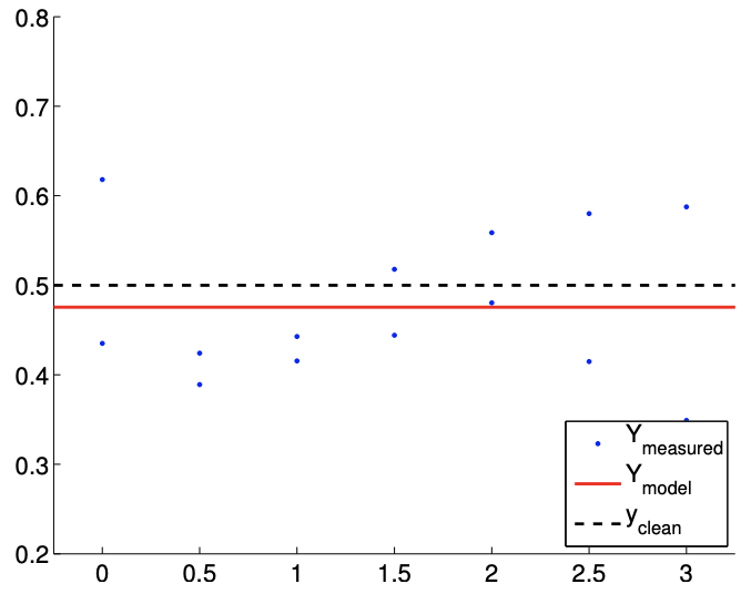
(a) \(m=14\)

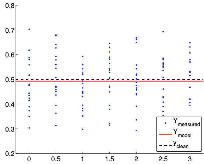
(b) \(m=140\)

Figure 19.2: Least square fitting of a constant function using a constant model.

Our confidence in the estimator \(\hat{\beta}_{0}\) converges as \(1 / \sqrt{m}=m^{-1 / 2}\). Again, the convergence rate is identical to that in Chapter \(11 .\)

As an example, consider a random function of the form \[Y \sim \frac{1}{2}+\mathcal{N}\left(0, \sigma^{2}\right),\] with the variance \(\sigma^{2}=0.01\), and a constant (polynomial) response model, i.e. \[Y_{\operatorname{model}}(x ; \beta)=\beta_{0}\] Note that the true parameter is given by \(\beta_{0}^{\text {true }}=1 / 2\). Our objective is to compute the least-squares estimate of \(\beta_{0}^{\text {true }}, \hat{\beta}_{0}\), and the associated confidence interval estimate, \(I_{0}\). We take measurements at seven points, \(x=0,0.5,1.0, \ldots, 3.0 ;\) at each point we take \(n_{\text {sample}}\) measurements for the total of \(m = 7 \cdot n_{\text{sample}}\) measurements. Several measurements (or replication) at the same \(x\) can be advantageous, as we will see shortly; however it is also possible in particular thanks to our homoscedastic assumption to take only a single measurement at each value of \(x\).

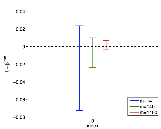
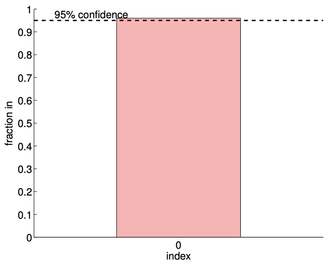
The results of the least squares fitting for \(m=14\) and \(m=140\) are shown in Figure \(19.2\). Here \(y_{\text {clean }}\) corresponds to the noise-free data, \(y_{\text {clean }}=1 / 2\). The convergence of the \(95 \%\) confidence interval with number of samples is depicted in Figure \(19.3(\mathrm{a})\). We emphasize that for the purpose of these figures and later similar figures we plot the confidence intervals shifted by \(\beta_{0}^{\text {true }}\). We would not know \(\beta_{0}^{\text {true }}\) in practice, however these figures are intended to demonstrate the performance of the confidence intervals in a case in which the true values are indeed known. Each of the realizations of the confidence intervals includes the true parameter value. In fact, for the \(m=140\) case, Figure \(19.3(\mathrm{~b})\) shows that 96 out of 100 realizations of the confidence interval include the true parameter value, which is consistent with the \(95 \%\) confidence level for the interval. (Of course in practice we would compute only a single confidence interval.)

(a) \(95 \%\) shifted confidence intervals

(b) \(95 \% \mathrm{ci}\) in/out (100 realizations, \(m=140)\)

Figure 19.3: (a) The variation in the \(95 \%\) confidence interval with the sampling size \(m\) for the constant model fitting. (b) The frequency of the confidence interval \(I_{0}\) including the true parameter \(\beta_{0}^{\text {true }} .\)

Example 19.1.3 constant regression model and its relation to deterministic analysis

Earlier, we studied how a data perturbation \(g-g_{0}\) affects the least squares solution \(z^{*}-z_{0}\). In the analysis we assumed that there is a unique solution \(z_{0}\) to the clean problem, \(B z_{0}=g_{0}\), and then compared the solution to the least squares solution \(z^{*}\) to the perturbed problem, \(B z^{*}=g\). As in the previous analysis, we use subscript 0 to represent superscript "true" to declutter the notation.

Now let us consider a statistical context, where the perturbation in the right-hand side is induced by the zero-mean normal distribution with variance \(\sigma^{2}\). In this case, \[\frac{1}{m} \sum_{i=1}^{m}\left(g_{0, i}-g_{i}\right)\] is the sample mean of the normal distribution, which we expect to incur fluctuations on the order of \(\sigma / \sqrt{m}\). In other words, the deviation in the solution is \[z_{0}-z^{*}=\left(B^{\mathrm{T}} B\right)^{-1} B^{\mathrm{T}}\left(g_{0}-g\right)=m^{-1} \sum_{i=1}^{m}\left(g_{0, i}-g_{i}\right)=\mathcal{O}\left(\frac{\sigma}{\sqrt{m}}\right)\] Note that this convergence is faster than that obtained directly from the earlier perturbation bounds, \[\left|z_{0}-z^{*}\right| \leq \frac{1}{\sqrt{m}}\left\|g_{0}-g\right\|=\frac{1}{\sqrt{m}} \sqrt{m} \sigma=\sigma\] which suggests that the error would not converge. The difference suggests that the perturbation resulting from the normal noise is different from any arbitrary perturbation. In particular, recall that the deterministic bound based on the Cauchy-Schwarz inequality is pessimistic when the perturbation is not well aligned with \(\operatorname{col}(B)\), which is a constant. In the statistical context, the noise \(g_{0}-g\) is relatively orthogonal to the column space \(\operatorname{col}(B)\), resulting in a faster convergence than for an arbitrary perturbation.

(a) \(m=14\)

(b) \(m=140\)

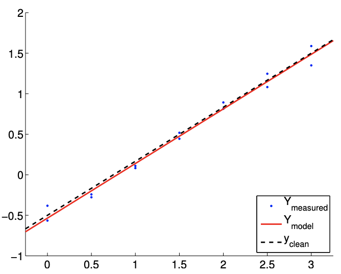
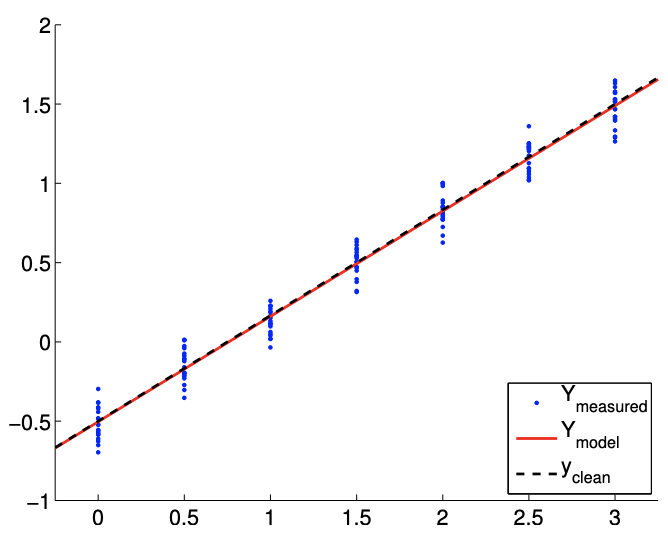
Figure 19.4: Least square fitting of a linear function using a linear model.

Example 19.1.4 least-squares estimate for a linear model

As the second example, consider a random function of the form \[Y(x) \sim-\frac{1}{2}+\frac{2}{3} x+\mathcal{N}\left(0, \sigma^{2}\right),\] with the variance \(\sigma^{2}=0.01\). The objective is to model the function using a linear model \[Y_{\text {model }}(x ; \beta)=\beta_{0}+\beta_{1} x\] where the parameters \(\left(\beta_{0}, \beta_{1}\right)\) are found through least squares fitting. Note that the true parameters are given by \(\beta_{0}^{\text {true }}=-1 / 2\) and \(\beta_{1}^{\text {true }}=2 / 3\). As in the constant model case, we take measurements at seven points, \(x=0,0.5,1.0, \ldots, 3.0\); at each point we take \(n_{\text {sample measurements for the total }}\) of \(m=7 \cdot n_{\text {sample }}\) measurements. Here, it is important that we take measurements at at least two different \(x\) locations; otherwise, the matrix \(B\) will be singular. This makes sense because if we choose only a single \(x\) location we are effectively trying to fit a line through a single point, which is an ill-posed problem.

The results of the least squares fitting for \(m=14\) and \(m=140\) are shown in Figure \(19.4\). We see that the fit gets tighter as the number of samples, \(m\), increases.

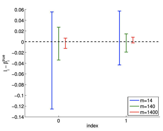
We can also quantify the quality of the parameter estimation in terms of the confidence intervals. The convergence of the individual \(95 \%\) confidence interval with number of samples is depicted in Figure \(19.5(\mathrm{a})\). Recall that the individual confidence intervals, \(I_{i}, i=0,1\), are constructed to satisfy \[P\left(\beta_{0}^{\text {true }} \in I_{0}\right)=\gamma \quad \text { and } \quad P\left(\beta_{1}^{\text {true }} \in I_{1}\right)=\gamma\] with the confidence level \(\gamma(95 \%\) for this case) using the Student’s \(t\)-distribution. Clearly each of the individual confidence intervals gets tighter as we take more measurements and our confidence in our parameter estimate improves. Note that the realization of confidence intervals include the true parameter value for each of the sample sizes considered.

(a) \(95 \%\) shifted confidence intervals

(b) \(95 \% \mathrm{ci}\) in/out ( 1000 realizations, \(m=140)\)

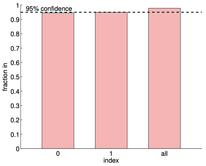
Figure 19.5: a) The variation in the \(95 \%\) confidence interval with the sampling size \(m\) for the linear model fitting. b) The frequency of the individual confidence intervals \(I_{0}\) and \(I_{1}\) including the true parameters \(\beta_{0}^{\text {true }}\) and \(\beta_{1}^{\text {true }}\left(0\right.\) and 1 , respectively), and \(I_{0}^{\text {joint }} \times I_{1}^{\text {joint }}\) jointly including ( \(\left.\beta_{0}^{\text {true }}, \beta_{1}^{\text {true }}\right)\) (all).

We can verify the validity of the individual confidence intervals by measuring the frequency that each of the true parameters lies in the corresponding interval for a large number of realizations. The result for 1000 realizations is shown in Figure 19.5(b). The column indexed "0" corresponds to the frequency of \(\beta_{0}^{\text {true }} \in I_{0}\), and the column indexed "1" corresponds to the frequency of \(\beta_{1}^{\text {true }} \in I_{1}\). As designed, each of the individual confidence intervals includes the true parameter \(\gamma=95 \%\) of the times.

We can also check the validity of the joint confidence interval by measuring the frequency that the parameters \(\left(\beta_{1}, \beta_{2}\right)\) jointly takes on values within \(I_{0}^{\text {joint }} \times I_{1}^{\text {joint }}\). Recall that the our joint intervals are designed to satisfy \[P\left(\beta_{0}^{\text {true }} \in I_{0}^{\text {joint }} \text { and } \beta_{1}^{\text {true }} \in I_{1}^{\text {joint }}\right) \geq \gamma\] and it uses the \(F\)-distribution. The column indexed "all" in Figure 19.5(b). corresponds to the frequency that \(\left(\beta_{0}^{\text {true }}, \beta_{1}^{\text {true }}\right) \in I_{0}^{\text {joint }} \times I_{1}^{\text {joint }}\). Note that the joint success rate is a slightly higher \((\approx 97 \%)\) than \(\gamma\) since the confidence intervals we provide are a simple but conservative bound for the actual elliptical confidence region. On the other hand, if we mistakenly use the individual confidence intervals instead of the joint confidence interval, the individual confidence intervals are too small and jointly include the true parameters only \(\approx 92 \%\) of the time. Thus, we emphasize that it is important to construct confidence intervals that are appropriate for the question of interest.

Hypothesis Testing

We can also, in place of our CI’s (or in fact, based on our CI’s), consider a hypotheses on the parameters - and then test these hypotheses. For example, in this last example, we might wish to test the hypothesis (known as the null hypothesis) that \(\beta_{0}^{\text {true }}=0\). We consider Example 19.1.4 for the case in which \(m=1400\). Clearly, our CI does not include \(\beta_{0}^{\text {true }}=0\). Thus most likely \(\beta_{0}^{\text {true }} \neq 0\), and we reject the hypothesis. In general, we reject the hypothesis when the CI does not include zero.

We can easily analyze the Type I error, which is defined as the probability that we reject the hypothesis when the hypothesis is in fact true. We assume the hypothesis is true. Then, the probability that the CI does not include zero - and hence that we reject the hypothesis - is \(0.05\), since we know that \(95 \%\) of the time our CI will include zero - the true value under our hypothesis. (This can be rephrased in terms of a test statistic and a critical region for rejection.) We denote by \(0.05\) the "size" of the test - the probability that we incorrectly reject the hypothesis due to an unlucky (rare) "fluctuation."

We can also introduce the notion of a Type II error, which is defined as the probability that we accept the hypothesis when the hypothesis is in fact false. And the "power" of the test is the probability that we reject the hypothesis when the hypothesis in fact false: the power is 1 - the Type II error. Typically it is more difficult to calculate Type II errors (and power) than Type I errors.

Inspection of Assumptions

In estimating the parameters for the response model and constructing the corresponding confidence intervals, we relied on the noise assumptions (N1), (N2), and (N3). In this section, we consider examples that illustrate how the assumptions may be broken. Then, we propose methods for verifying the plausibility of the assumptions. Note we give here some rather simple tests without any underlying statistical structure; in fact, it is possible to be more rigorous about when to accept or reject our noise and bias hypotheses by introducing appropriate statistics such that "small" and "large" can be quantified. (It is also possible to directly pursue our parameter estimation under more general noise assumptions.)

Checking for Plausibility of the Noise Assumptions

Let us consider a system governed by a random affine function, but assume that the noise \(\epsilon(x)\) is perfectly correlated in \(x\). That is, \[Y\left(x_{i}\right)=\beta_{0}^{\text {true }}+\beta_{1}^{\text {true }} x_{i}+\epsilon\left(x_{i}\right),\] where \[\epsilon\left(x_{1}\right)=\epsilon\left(x_{2}\right)=\cdots=\epsilon\left(x_{m}\right) \sim \mathcal{N}\left(0, \sigma^{2}\right) .\] Even though the assumptions (N1) and (N2) are satisfied, the assumption on independence, (N3), is violated in this case. Because the systematic error shifts the output by a constant, the coefficient of the least-squares solution corresponding to the constant function \(\beta_{0}\) would be shifted by the error. Here, the (perfectly correlated) noise \(\epsilon\) is incorrectly interpreted as signal.

Let us now present a test to verify the plausibility of the assumptions, which would detect the presence of the above scenario (amongst others). The verification can be accomplished by sampling the system in a controlled manner. Say we gather \(N\) samples evaluated at \(x_{L}\), \[L_{1}, L_{2}, \ldots, L_{N} \quad \text { where } \quad L_{i}=Y\left(x_{L}\right), \quad i=1, \ldots, N .\] Similarly, we gather another set of \(N\) samples evaluated at \(x_{R} \neq x_{L}\), \[R_{1}, R_{2}, \ldots, R_{N} \quad \text { where } \quad R_{i}=Y\left(x_{R}\right), \quad i=1, \ldots, N .\] Using the samples, we first compute the estimate for the mean and variance for \(L\), \[\hat{\mu}_{L}=\frac{1}{N} \sum_{i=1}^{N} L_{i} \quad \text { and } \quad \hat{\sigma}_{L}^{2}=\frac{1}{N-1} \sum_{i=1}^{N}\left(L_{i}-\hat{\mu}_{L}\right)^{2},\] and those for \(R\), \[\hat{\mu}_{R}=\frac{1}{N} \sum_{i=1}^{N} R_{i} \quad \text { and } \quad \hat{\sigma}_{R}^{2}=\frac{1}{N-1} \sum_{i=1}^{N}\left(R_{i}-\hat{\mu}_{R}\right)^{2} .\] To check for the normality assumption (N1), we can plot the histogram for \(L\) and \(R\) (using an appropriate number of bins) and for \(\mathcal{N}\left(\hat{\mu}_{L}, \hat{\sigma}_{L}^{2}\right)\) and \(\mathcal{N}\left(\hat{\mu}_{R}, \hat{\sigma}_{R}^{2}\right)\). If the error is normally distributed, these histograms should be similar, and resemble the normal distribution. In fact, there are much more rigorous and quantitative statistical tests to assess whether data derives from a particular (here normal) population.

To check for the homoscedasticity assumption (N2), we can compare the variance estimate for samples \(L\) and \(R\), i.e., is \(\hat{\sigma}_{L}^{2} \approx \hat{\sigma}_{R}^{2}\) ? If \(\hat{\sigma}_{L}^{2} \approx \hat{\sigma}_{R}^{2}\), then assumption (N2) is not likely plausible because the noise at \(x_{L}\) and \(x_{R}\) have different distributions.

Finally, to check for the uncorrelatedness assumption (N3), we can check the correlation coefficient \(\rho_{L, R}\) between \(L\) and \(R\). The correlation coefficient is estimated as \[\hat{\rho}_{L, R}=\frac{1}{\hat{\sigma}_{L} \hat{\sigma}_{R}} \frac{1}{N-1} \sum_{i=1}^{N}\left(L_{i}-\hat{\mu}_{L}\right)\left(R_{i}-\hat{\mu}_{R}\right) .\] If the correlation coefficient is not close to 0 , then the assumption (N3) is not likely plausible. In the example considered with the correlated noise, our system would fail this last test.

Checking for Presence of Bias

Let us again consider a system governed by an affine function. This time, we assume that the system is noise free, i.e. \[Y(x)=\beta_{0}^{\text {true }}+\beta_{1}^{\text {true }} x\] We will model the system using a constant function, \[Y_{\text {model }}=\beta_{0} .\] Because our constant model would match the mean of the underlying distribution, we would interpret \(Y\) - mean \((Y)\) as the error. In this case, the signal is interpreted as a noise.

We can check for the presence of bias by checking if \[\left|\hat{\mu}_{L}-\widehat{Y}_{\text {model }}\left(x_{L}\right)\right| \sim \mathcal{O}(\hat{\sigma}) .\] If the relationship does not hold, then it indicates a lack of fit, i.e., the presence of bias. Note that replication - as well as data exploration more generally - is crucial in understanding the assumptions. Again, there are much more rigorous and quantitative statistical (say, hypothesis) tests to assess whether bias is present.