19.2: General Case

We consider a more general case of regression, in which we do not restrict ourselves to a linear response model. However, we still assume that the noise assumptions (N1), (N2), and (N3) hold.

Response Model

Consider a general relationship between the measurement \(Y\), response model \(Y_{\text {model }}\), and the noise \(\epsilon\) of the form \[Y(x)=Y_{\text {model }}(x ; \beta)+\epsilon,\] where the independent variable \(x\) is vector valued with \(p\) components, i.e. \[x=\left(x_{(1)}, x_{(2)}, \cdots, x_{(p)}\right)^{\mathrm{T}} \in D \subset \mathbb{R}^{p} .\] The response model is of the form \[Y_{\text {model }}(x ; \beta)=\beta_{0}+\sum_{j=1}^{n-1} \beta_{j} h_{j}(x),\] where \(h_{j}, j=0, \ldots, n-1\), are the basis functions and \(\beta_{j}, j=0, \ldots, n-1\), are the regression coefficients. Note that we have chosen \(h_{0}(x)=1\). Similar to the affine case, we assume that \(Y_{\text {model }}\) is sufficiently rich (with respect to the underlying random function \(Y\) ), such that there exists a parameter \(\beta^{\text {true }}\) with which \(Y_{\text {model }}\left(\cdot ; \beta^{\text {true }}\right)\) perfectly describes the behavior of the noise-free underlying function, i.e., unbiased. (Equivalently, there exists a \(\beta^{\text {true }}\) such that \(Y(x) \sim \mathcal{N}\left(Y_{\text {model }}\left(x ; \beta^{\text {true }}\right), \sigma^{2}\right)\).

It is important to note that this is still a linear regression. It is linear in the sense that the regression coefficients \(\beta_{j}, j=0, \ldots, n-1\), appear linearly in \(Y_{\text {model }}\). The basis functions \(h_{j}\), \(j=0, \ldots, n-1\), do not need to be linear in \(x\); for example, \(h_{1}\left(x_{(1)}, x_{(2)}, x_{(3)}\right)=x_{(1)} \exp \left(x_{(2)} x_{(3)}\right)\) is perfectly acceptable for a basis function. The simple case considered in the previous section corresponds to \(p=1, n=2\), with \(h_{0}(x)=1\) and \(h_{1}(x)=x\).

There are two main approaches to choose the basis functions.

(i) Functions derived from anticipated behavior based on physical models. For example, to deduce the friction coefficient, we can relate the static friction and the normal force following the Amontons’ and Coulomb’s laws of friction, \[F_{\mathrm{f}, \text { static }}=\mu_{\mathrm{s}} F_{\text {normal, applied }}\] where \(F_{\mathrm{f}, \text { static }}\) is the friction force, \(\mu_{\mathrm{s}}\) is the friction coefficient, and \(F_{\text {normal, applied is the normal }}\) force. Noting that \(F_{\mathrm{f} \text {, static }}\) is a linear function of \(F_{\text {normal, applied, we can choose a linear basis }}\) function \(h_{1}(x)=x\).

Although we can choose \(n\) large and let least-squares find the \(\operatorname{good} \beta\) - the good model within our general expansion - this is typically not a good idea: to avoid overfitting, we must ensure the number of experiments is much greater than the order of the model, i.e., \(m \gg n\). We return to overfitting later in the chapter.

Estimation

We take \(m\) measurements to collect \(m\) independent variable-measurement pairs \[\left(x_{i}, Y_{i}\right), \quad i=1, \ldots, m,\] where \(x_{i}=\left(x_{(1)}, x_{(2)}, \ldots, x_{(p)}\right)_{i}\). We claim \[\begin{aligned} Y_{i} &=Y_{\text {model }}\left(x_{i} ; \beta\right)+\epsilon_{i} \\ &=\beta_{0}+\sum_{j=1}^{n-1} \beta_{j} h_{j}\left(x_{i}\right)+\epsilon_{i}, \quad i=1, \ldots, m, \end{aligned}\] which yields \[\underbrace{\left(\begin{array}{c} Y_{1} \\ Y_{2} \\ \vdots \\ Y_{m} \end{array}\right)}_{Y}=\underbrace{\left(\begin{array}{ccccc} 1 & h_{1}\left(x_{1}\right) & h_{2}\left(x_{1}\right) & \ldots & h_{n-1}\left(x_{1}\right) \\ 1 & h_{1}\left(x_{2}\right) & h_{2}\left(x_{2}\right) & \ldots & h_{n-1}\left(x_{2}\right) \\ \vdots & \vdots & \vdots & \vdots & \vdots \\ 1 & h_{1}\left(x_{m}\right) & h_{2}\left(x_{m}\right) & \ldots & h_{n-1}\left(x_{m}\right) \end{array}\right)}_{X} \underbrace{\left(\begin{array}{c} \beta_{0} \\ \beta_{1} \\ \vdots \\ \beta_{n-1} \end{array}\right)}_{\beta}+\underbrace{\left(\begin{array}{c} \epsilon\left(x_{1}\right) \\ \epsilon\left(x_{2}\right) \\ \vdots \\ \epsilon\left(x_{m}\right) \end{array}\right)}_{\epsilon} .\] The least-squares estimator \(\hat{\beta}\) is given by \[\left(X^{\mathrm{T}} X\right) \hat{\beta}=X^{\mathrm{T}} Y,\] and the goodness of fit is measured by \(\hat{\sigma}\), \[\hat{\sigma}=\left(\frac{1}{m-n}\|Y-\widehat{Y}\|^{2}\right)^{1 / 2},\] where \[\widehat{Y}=\left(\begin{array}{c} \widehat{Y}_{\text {model }}\left(x_{1}\right) \\ \widehat{Y}_{\text {model }}\left(x_{2}\right) \\ \vdots \\ \widehat{Y}_{\text {model }}\left(x_{m}\right) \end{array}\right)=\left(\begin{array}{c} \hat{\beta}_{0}+\sum_{j=1}^{n-1} \hat{\beta}_{j} h_{j}\left(x_{1}\right) \\ \hat{\beta}_{0}+\sum_{j=1}^{n-1} \hat{\beta}_{j} h_{j}\left(x_{2}\right) \\ \vdots \\ \hat{\beta}_{0}+\sum_{j=1}^{n-1} \hat{\beta}_{j} h_{j}\left(x_{m}\right) \end{array}\right)=X \hat{\beta} .\] As before, the mean of the mean of the model is equal to the mean of the measurements, i.e. \[\overline{\widehat{Y}}=\bar{Y}\] where \[\overline{\widehat{Y}}=\frac{1}{m} \sum_{i=1}^{m} \widehat{Y}_{i} \text { and } \bar{Y}=\frac{1}{m} \sum_{i=1}^{m} Y_{i} .\] The preservation of the mean is ensured by the presence of the constant term \(\beta_{0} \cdot 1\) in our model.

Confidence Intervals

The construction of the confidence intervals follows the procedure developed in the previous section. Let us define the covariance matrix \[\widehat{\Sigma}=\hat{\sigma}^{2}\left(X^{\mathrm{T}} X\right)^{-1}\] Then, the individual confidence intervals are given by \[I_{j}=\left[\hat{\beta}_{j}-t_{\gamma, m-n} \sqrt{\widehat{\Sigma}_{j+1, j+1}}, \hat{\beta}_{j}+t_{\gamma, m-n} \sqrt{\widehat{\Sigma}_{j+1, j+1}}\right], \quad j=0, \ldots, n-1,\] where \(t_{\gamma, m-n}\) comes from the Student’s \(t\)-distribution as before, i.e. \[t_{\gamma, m-n}=F_{T, m-n}^{-1}\left(\frac{1}{2}+\frac{\gamma}{2}\right),\] where \(F_{T, q}^{-1}\) is the inverse cumulative distribution function of the \(t\)-distribution. The shifting of the covariance matrix indices is due to the index for the parameters starting from 0 and the index for the matrix starting from 1. Each of the individual confidence intervals satisfies \[P\left(\beta_{j}^{\text {true }} \in I_{j}\right)=\gamma, \quad j=0, \ldots, n-1,\] where \(\gamma\) is the confidence level.

We can also develop joint confidence intervals, \[I_{j}^{\text {joint }}=\left[\hat{\beta}_{j}-s_{\gamma, n, m-n} \sqrt{\widehat{\Sigma}_{j+1, j+1}}, \hat{\beta}_{j}+s_{\gamma, n, m-n} \sqrt{\widehat{\Sigma}_{j+1, j+1}}\right], \quad j=0, \ldots, n-1,\] where the parameter \(s_{\gamma, n, m-n}\) is calculated from the inverse cumulative distribution function for the \(F\)-distribution according to \[s_{\gamma, n, m-n}=\sqrt{n F_{F, n, m-n}^{-1}(\gamma)} .\] The joint confidence intervals satisfy \[P\left(\beta_{0}^{\text {true }} \in I_{0}^{\text {joint }}, \beta_{1}^{\text {true }} \in I_{1}^{\text {joint }}, \ldots, \beta_{n-2}^{\text {true }} \in I_{n-2}^{\text {joint }}, \text { and } \beta_{n-1}^{\text {true }} \in I_{n-1}^{\text {joint }}\right) \geq \gamma .\]

Example 19.2.1 least-squares estimate for a quadratic function

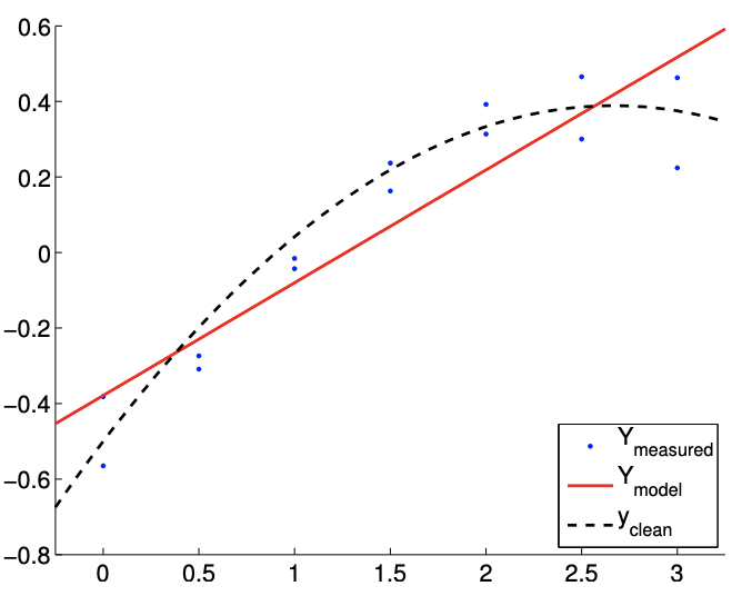
Consider a random function of the form \[Y(x) \sim-\frac{1}{2}+\frac{2}{3} x-\frac{1}{8} x^{2}+\mathcal{N}\left(0, \sigma^{2}\right),\] with the variance \(\sigma^{2}=0.01\). We would like to model the behavior of the function. Suppose we know (though a physical law or experience) that the output of the underlying process depends quadratically on input \(x\). Thus, we choose the basis functions \[h_{1}(x)=1, \quad h_{2}(x)=x, \quad \text { and } \quad h_{3}(x)=x^{2} .\] The resulting model is of the form \[Y_{\text {model }}(x ; \beta)=\beta_{0}+\beta_{1} x+\beta_{2} x^{2},\]

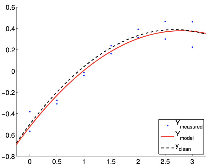
(a) \(m=14\)

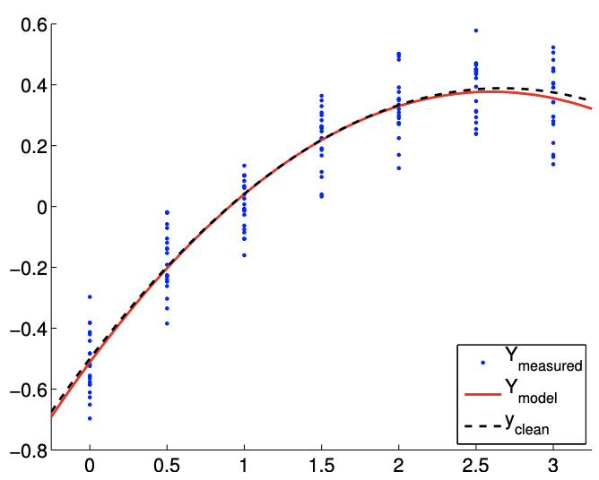
(b) \(m=140\)

Figure 19.6: Least squares fitting of a quadratic function using a quadratic model.

where \(\left(\beta_{0}, \beta_{1}, \beta_{2}\right)\) are the parameters to be determined through least squares fitting. Note that the true parameters are given by \(\beta_{0}^{\text {true }}=-1 / 2, \beta_{1}^{\text {true }}=2 / 3\), and \(\beta_{2}^{\text {true }}=-1 / 8\).

The result of the calculation is shown in Figure 19.6. Our model qualitatively matches well with the underlying "true" model. Figure \(19.7(\mathrm{a})\) shows that the \(95 \%\) individual confidence interval for each of the parameters converges as the number of samples increase.

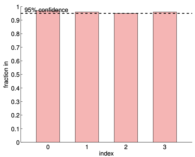
Figure 19.7(b) verifies that the individual confidence intervals include the true parameter approximately \(95 \%\) of the times (shown in the columns indexed 0,1 , and 2). Our joint confidence interval also jointly include the true parameter about \(98 \%\) of the times, which is greater than the prescribed confidence level of \(95 \%\). (Note that individual confidence intervals jointly include the true parameters only about \(91 \%\) of the times.) These results confirm that both the individual and joint confidence intervals are reliable indicators of the quality of the respective estimates.

Overfitting (and Underfitting)

We have discussed the importance of choosing a model with a sufficiently large \(n-\) such that the true underlying distribution is representable and there would be no bias - but also hinted that \(n\) much larger than necessary can result in an overfitting of the data. Overfitting significantly degrades the quality of our parameter estimate and predictive model, especially when the data is noisy or the number of data points is small. Let us illustrate the effect of overfitting using a few examples.

Example 19.2.2 overfitting of a linear function

Let us consider a noisy linear function \[Y(x) \sim \frac{1}{2}+2 x+\mathcal{N}\left(0, \sigma^{2}\right) .\] However, unlike in the previous examples, we assume that we do not know the form of the inputoutput dependency. In this and the next two examples, we will consider a general \(n-1\) degree polynomial fit of the form \[Y_{\text {model }, n}(x ; \beta)=\beta_{0}+\beta_{1} x^{1}+\cdots+\beta_{n-1} x^{n-1} .\]

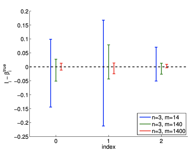
(a) \(95 \%\) shifted confidence intervals

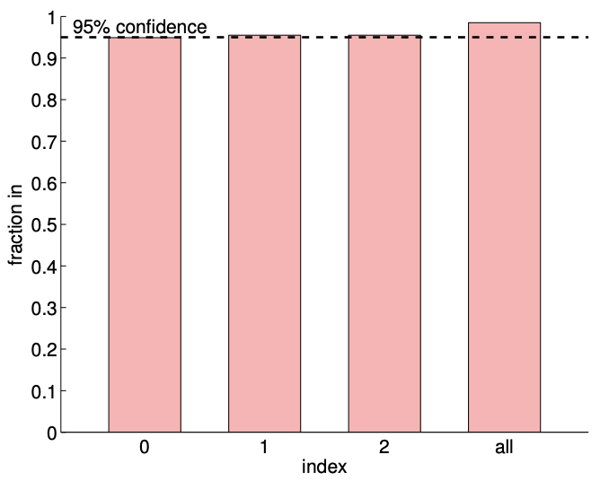
(b) \(95 \% \mathrm{ci}\) in/out ( 1000 realizations, \(m=140)\)

Figure 19.7: (a) The variation in the \(95 \%\) confidence interval with the sampling size \(m\) for the linear model fitting. (b) The frequency of the individual confidence intervals \(I_{0}, I_{1}\), and \(I_{2}\) including the true parameters \(\beta_{0}^{\text {true }}, \beta_{1}^{\text {true }}\), and \(\beta_{2}^{\text {true }}\left(0,1\right.\), and 2 , respectively), and \(I_{0}^{j \text { joint }} \times I_{1}^{\text {joint }} \times I_{2}^{\text {joint }}\) jointly including \(\left(\beta_{0}^{\text {true }}, \beta_{1}^{\text {true }}, \beta_{2}^{\text {true }}\right)\) (all).

Note that the true parameters for the noisy function are \[\beta_{0}^{\text {true }}=\frac{1}{2}, \quad \beta_{1}^{\text {true }}=2, \quad \text { and } \quad \beta_{2}^{\text {true }}=\cdots=\beta_{n}^{\text {true }}=0\] for any \(n \geq 2\).

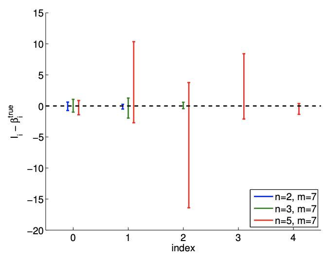
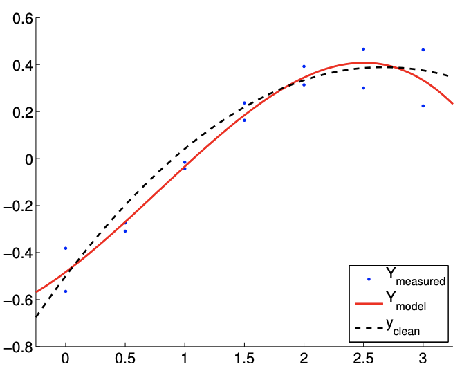
The results of fitting the noisy linear function using \(m=7\) measurements for the \(n=2, n=3\), and \(n=5\) response models are shown in Figure \(19.8(\mathrm{a}),(\mathrm{b})\), and \((\mathrm{c})\), respectively. The \(n=2\) is the nominal case, which matches the true underlying functional dependency, and the \(n=3\) and \(n=5\) cases correspond to overfitting cases. For each fit, we also state the least-squares estimate of the parameters. Qualitatively, we see that the prediction error, \(y_{\text {clean }}(x)-Y_{\text {model }}(x)\), is larger for the quartic model \((n=5)\) than the affine model \((n=2)\). In particular, because the quartic model is fitting five parameters using just seven data points, the model is close to interpolating the noise, resulting in an oscillatory behavior that follows the noise. This oscillation becomes more pronounced as the noise level, \(\sigma\), increases.

In terms of estimating the parameters \(\beta_{0}^{\text {true }}\) and \(\beta_{1}^{\text {true }}\), the affine model again performs better than the overfit cases. In particular, the error in \(\hat{\beta}_{1}\) is over an order of magnitude larger for the \(n=5\) model than for the \(n=2\) model. Fortunately, this inaccuracy in the parameter estimate is reflected in large confidence intervals, as shown in Figure \(19.9\). The confidence intervals are valid because our models with \(n \geq 2\) are capable of representing the underlying functional dependency with \(n^{\text {true }}=2\), and the unbiasedness assumption used to construct the confidence intervals still holds. Thus, while the estimate may be poor, we are informed that we should not have much confidence in our estimate of the parameters. The large confidence intervals result from the fact that overfitting effectively leaves no degrees of freedom (or information) to estimate the noise because relatively too many degrees of freedom are used to determine the parameters. Indeed, when \(m=n\), the confidence intervals are infinite.

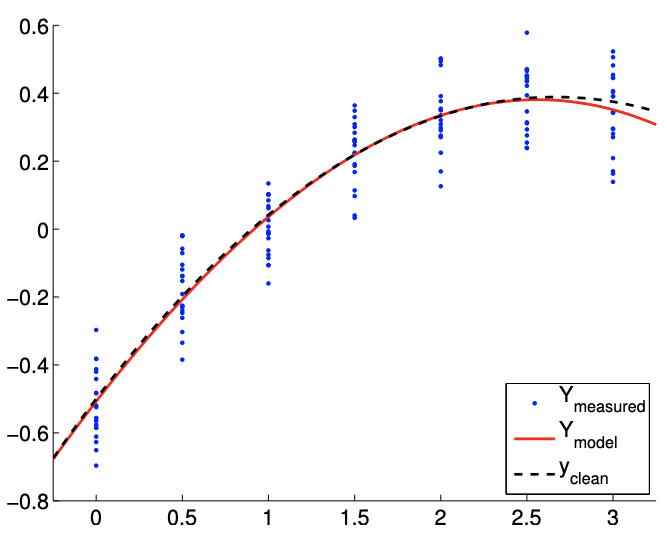
Because the model is unbiased, more data ultimately resolves the poor fit, as shown in Figure \(19.8(\mathrm{~d})\). However, recalling that the confidence intervals converge only as \(m{ }^{-1 / 2}\), a large

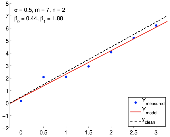
(a) \(m=7, n=2\)

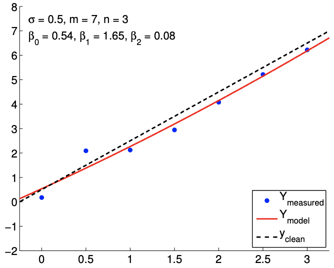
(b) \(m=7, n=3\)

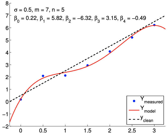
(c) \(m=7, n=5\)

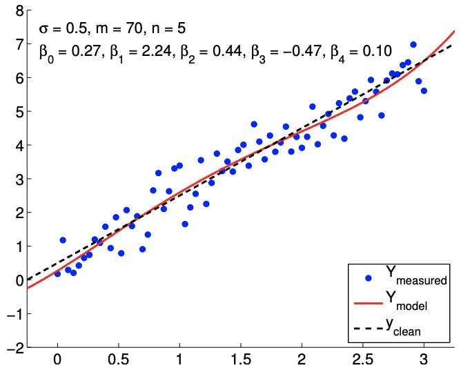
(d) \(m=70, n=5\)

Figure 19.8: Least squares fitting of a linear function using polynomial models of various orders.

Figure 19.9: The \(95 \%\) shifted confidence intervals for fitting a linear function using polynomial models of various orders.

number of samples are required to tighten the confidence intervals - and improve our parameter estimates - for the overfitting cases. Thus, deducing an appropriate response model based on, for example, physical principles can significantly improve the quality of the parameter estimates and the performance of the predictive model.

Begin Advanced Material

Example 19.2.3 overfitting of a quadratic function

In this example, we study the effect of overfitting in more detail. We consider data governed by a random quadratic function of the form \[Y(x) \sim-\frac{1}{2}+\frac{2}{3} x-\frac{1}{8} c x^{2}+\mathcal{N}\left(0, \sigma^{2}\right),\] with \(c=1\). We again consider for our model the polynomial form \(Y_{\text {model }, n}(x ; \beta)\).

Figure \(19.10\) (a) shows a typical result of fitting the data using \(m=14\) sampling points and \(n=4\). Our cubic model includes the underlying quadratic distribution. Thus there is no bias and our noise assumptions are satisfied. However, compared to the quadratic model \((n=3)\), the cubic model is affected by the noise in the measurement and produces spurious variations. This spurious variation tend to disappear with the number of sampling points, and Figure \(19.10\) (b) with \(m=140\) sampling points exhibits a more stable fit.

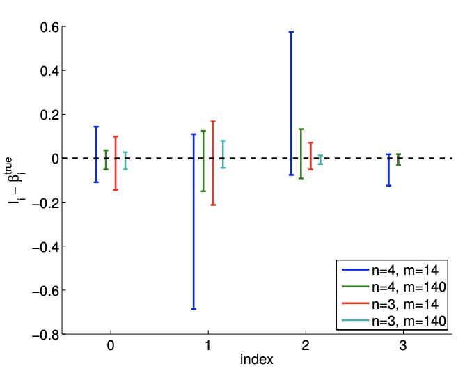
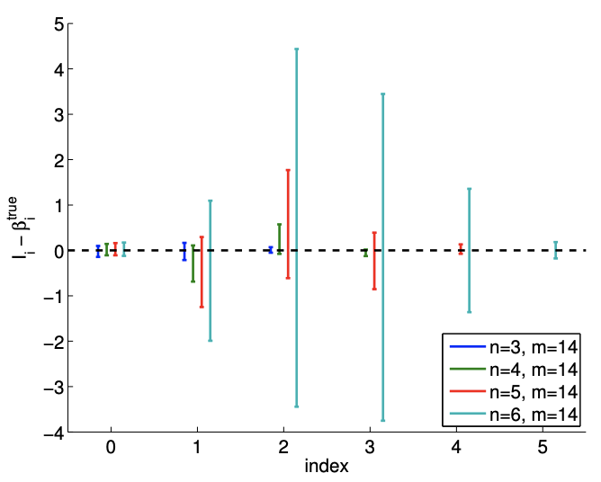
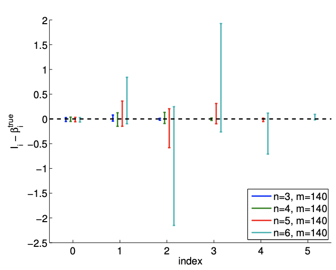
Figure \(19.10(\mathrm{c})\) shows a realization of confidence intervals for the cubic model \((n=4)\) using \(m=14\) and \(m=140\) sampling points. A realization of confidence intervals for the quadratic model ( \(n=3\) ) is also shown for comparison. Using the same set of data, the confidence intervals for the cubic model are larger than those of the quadratic model. However, the confidence intervals of the cubic model include the true parameter value for most cases. Figure \(19.10(\mathrm{~d})\) confirms that the \(95 \%\) of the realization of the confidence intervals include the true parameter. Thus, the confidence intervals are reliable indicators of the quality of the parameter estimates, and in general the intervals get tighter with \(m\), as expected. Modest overfitting, \(n=4\) vs. \(n=3\), with \(m\) sufficiently large, poses little threat.

Let us check how overfitting affects the quality of the fit using two different measures. The first is a measure of how well we can predict, or reproduce, the clean underlying function; the second is a measure for how well we approximate the underlying parameters.

First, we quantify the quality of prediction using the maximum difference in the model and the clean underlying data, \[e_{\max } \equiv \max _{x \in[-1 / 4,3+1 / 4]}\left|Y_{\text {model }, n}(x ; \hat{\beta})-Y_{\text {clean }}(x)\right| .\] Figure 19.11(a) shows the variation in the maximum prediction error with \(n\) for a few different values of \(m\). We see that we get the closest fit (in the sense of the maximum error), when \(n=3\) - when there are no "extra" terms in our model. When only \(m=7\) data points are used, the quality of the regression degrades significantly as we overfit the data \((n>3)\). As the dimension of the model \(n\) approaches the number of measurements, \(m\), we are effectively interpolating the noise. The interpolation induces a large error in the parameter estimates, and we can not estimate the noise since we are fitting the noise. We observe in general that the quality of the estimate improves as the number of samples is increased.

Second, we quantify the quality of the parameter estimates by measuring the error in the quadratic coefficient, i.e., \(\left|\beta_{2}-\hat{\beta}_{2}\right|\). Figure 19.11(b) shows that, not surprisingly, the error in the

(a) \(m=14\)

(b) \(m=140\)

(c) \(95 \%\) shifted confidence intervals

(d) \(95 \%\) ci in/out (100 realizations, \(m=140)\)

Figure 19.10: Least squares fitting of a quadratic function \((c=1)\) using a cubic model.

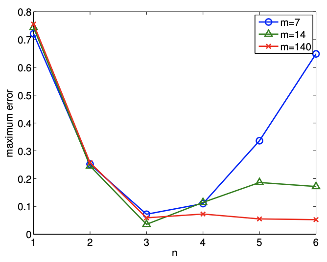
(a) maximum prediction error

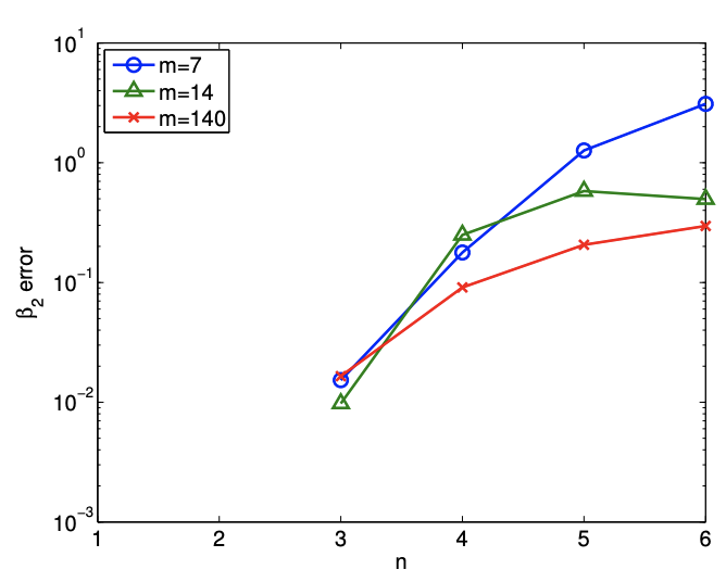
(b) error in parameter \(\beta_{2}\)

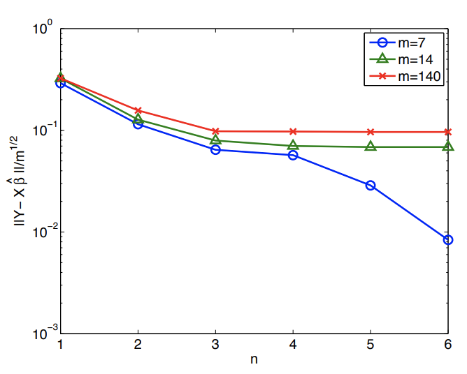
(c) (normalized) residual

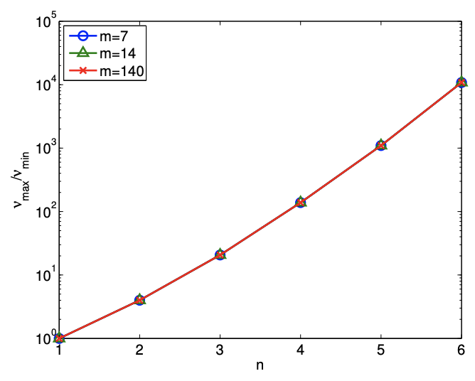
(d) condition number

Figure 19.11: Variation in the quality of regression with overfitting.

parameter increases under overfitting. In particular, for the small sample size of \(m=7\), the error in the estimate for \(\beta_{3}\) increases from \(\mathcal{O}\left(10^{-2}\right)\) for \(n=3\) to \(\mathcal{O}(1)\) for \(n \geq 5\). Since \(\beta_{3}\) is an \(\mathcal{O}(1)\) quantity, this renders the parameter estimates for \(n \geq 5\) essentially meaningless.

It is important to recognize that the degradation in the quality of estimate - either in terms of predictability or parameter error - is not due to the poor fit at the data points. In particular, the (normalized) residual, \[\frac{1}{m^{1 / 2}}\|Y-X \hat{\beta}\|,\] which measures the fit at the data points, decreases as \(n\) increases, as shown in Figure 19.11(c). The decrease in the residual is not surprising. We have new coefficients which were previously implicitly zero and hence the least squares must provide a residual which is non-increasing as we increase \(n\) and let these coefficients realize their optimal values (with respect to residual minimization). However, as we see in Figure 19.11(a) and 19.11(b), better fit at data points does not imply better representation of the underlying function or parameters.

The worse prediction of the parameter is due to the increase in the conditioning of the problem \(\left(\nu_{\max } / \nu_{\min }\right)\), as shown in Figure 19.11(d). Recall that the error in the parameter is a function of both residual (goodness of fit at \(\overline{\text { data points) and conditioning of the problem, i.e. }}\) \[\frac{\|\hat{\beta}-\beta\|}{\|\beta\|} \leq \frac{\nu_{\max }}{\nu_{\min }} \frac{\|X \hat{\beta}-Y\|}{\|Y\|} .\] As we increase \(n\) for a fixed \(m\), we do reduce the residual. However, clearly the error is larger both in terms of output prediction and parameter estimate. Once again we see that the residual - and similar commonly used goodness of fit statistics such as \(R^{2}\) - is not the "final answer" in terms of the success of any particular regression exercise.

Fortunately, similar to the previous example, this poor estimate of the parameters is reflected in large confidence intervals, as shown in Figure 19.12. Thus, while the estimates may be poor, we are informed that we should not have much confidence in our estimate of the parameters and that we need more data points to improve the fit.

Finally, we note that the conditioning of the problem reflects where we choose to make our measurements, our choice of response model, and how we choose to represent this response model. For example, as regards the latter, a Legendre (polynomial) expansion of order \(n\) would certainly decrease \(\nu_{\max } / \nu_{\min }\), albeit at some complication in how we extract various parameters of interest.

Example 19.2.4 underfitting of a quadratic function

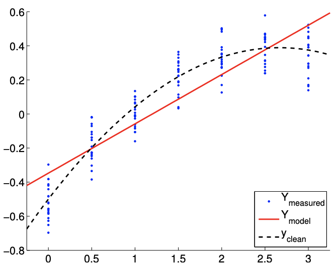
We consider data governed by a noisy quadratic function \(\left(n^{\text {true }} \equiv 3\right)\) of the form \[Y(x) \sim-\frac{1}{2}+\frac{2}{3} x-\frac{1}{8} c x^{2}+\mathcal{N}\left(0, \sigma^{2}\right) .\] We again assume that the input-output dependency is unknown. The focus of this example is underfitting; i.e., the case in which the degree of freedom of the model \(n\) is less than that of data \(n^{\text {true }}\). In particular, we will consider an affine model \((n=2)\), \[Y_{\text {model }, 2}(x ; \beta)=\beta_{0}+\beta_{1} x,\] which is clearly biased (unless \(c=0\) ).

For the first case, we consider the true underlying distribution with \(c=1\), which results in a strong quadratic dependency of \(Y\) on \(x\). The result of fitting the function is shown in Figure \(19.13\).

(a) \(m=14\)

(b) \(m=140\)

Figure 19.12: The variation in the confidence intervals for fitting a quadratic function using quadratic \((n=3)\), cubic \((n=4)\), quartic \((n=5)\), and quintic \((n=6)\) polynomials. Note the difference in the scales for the \(m=14\) and \(m=140\) cases.

Note that the affine model is incapable of representing the quadratic dependency even in the absence of noise. Thus, comparing Figure 19.13(a) and 19.13(b), the fit does not improve with the number of sampling points.

Figure 19.13(c) shows typical individual confidence intervals for the affine model \((n=2)\) using \(m=14\) and \(m=140\) sampling points. Typical confidence intervals for the quadratic model \((n=3)\) are also provided for comparison. Let us first focus on analyzing the fit of the affine model \((n=2)\) using \(m=14\) sampling points. We observe that this realization of confidence intervals \(I_{0}\) and \(I_{1}\) does not include the true parameters \(\beta_{0}^{\text {true }}\) and \(\beta_{1}^{\text {true }}\), respectively. In fact, Figure \(19.13(\mathrm{~d})\) shows that only 37 of the 100 realizations of the confidence interval \(I_{0}\) include \(\beta_{0}^{\text {true }}\) and that none of the realizations of \(I_{1}\) include \(\beta_{1}^{\text {true }}\). Thus the frequency that the true value lies in the confidence interval is significantly lower than \(95 \%\). This is due to the presence of the bias error, which violates our assumptions about the behavior of the noise - the assumptions on which our confidence interval estimate rely. In fact, as we increase the number of sampling point from \(m=14\) to \(m=140\) we see that the confidence intervals for both \(\beta_{0}\) and \(\beta_{1}\) tighten; however, they converge toward wrong values. Thus, in the presence of bias, the confidence intervals are unreliable, and their convergence implies little about the quality of the estimates.

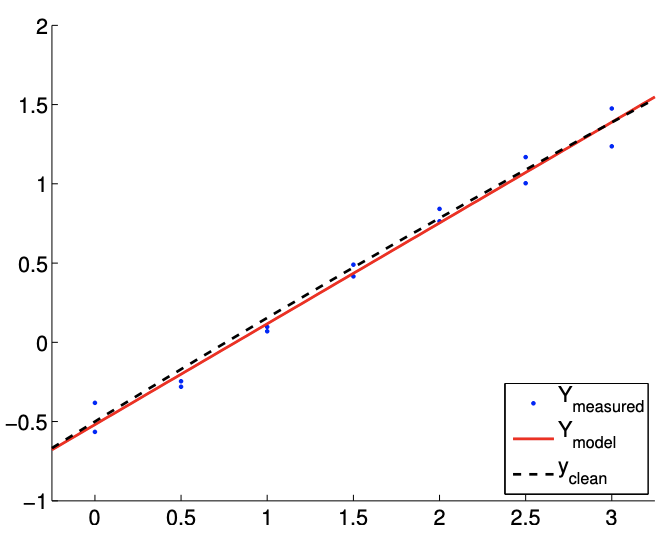
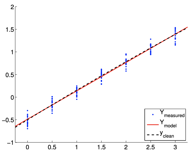
Let us now consider the second case with \(c=1 / 10\). This case results in a much weaker quadratic dependency of \(Y\) on \(x\). Typical fits obtained using the affine model are shown in Figure 19.14(a) and 19.14(b) for \(m=14\) and \(m=140\) sampling points, respectively. Note that the fit is better than the \(c=1\) case because the \(c=1 / 10\) data can be better represented using the affine model.

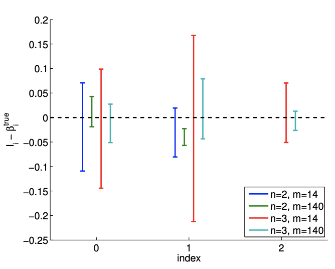
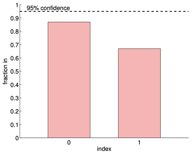
Typical confidence intervals, shown in Figure 19.14(c), confirm that the confidence intervals are more reliable than in the \(c=1\) case. Of the 100 realizations for the \(m=14\) case, \(87 \%\) and \(67 \%\) of the confidence intervals include the true values \(\beta_{0}^{\text {true }}\) and \(\beta_{1}^{\text {true }}\), respectively. The frequencies are lower than the \(95 \%\), i.e., the confidence intervals are not as reliable as their pretension, due to the presence of bias. However, they are more reliable than the case with a stronger quadratic dependence, i.e. a stronger bias. Recall that a smaller bias leading to a smaller error is consistent with the deterministic error bounds we developed in the presence of bias.

Similar to the \(c=1\) case, the confidence interval tightens with the number of samples \(m\), but

(a) \(m=14\)

(b) \(m=140\)

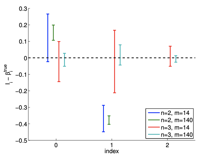
(c) \(95 \%\) shifted confidence intervals

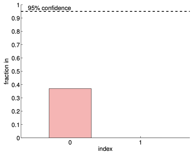
(d) \(95 \% \mathrm{ci} \mathrm{in/out}(100\) realizations, \(m=14)\)

Figure 19.13: Least squares fitting of a quadratic function \((c=1)\) using an affine model.

(a) \(m=14\)

(b) \(m=140\)

(c) \(95 \%\) shifted confidence intervals

(d) \(95 \% \mathrm{ci} \mathrm{in} /\) out ( 100 realizations, \(m=14)\)

Figure 19.14: Least squares fitting of a quadratic function \((c=1 / 10)\) using an affine model.

they converge to a wrong value. Accordingly, the reliability of the confidence intervals decreases with \(m\).

Advanced Material