
21.1: Scalar First-Order Linear ODEs
- Page ID
- 55693

Model Problem
Let us consider a canonical initial value problem (IVP),
\begin{aligned}
\frac{d u}{d t} &=\lambda u+f(t), \quad 0<t<t_{f} \\
u(0) &=u_{0}
\end{aligned}
The objective is to find \(u\) over all time \(t ∈ [0, t_f]\) that satisfies the ordinary differential equation (ODE) and the initial condition. This problem belongs to the class of initial value problems (IVP) since we supplement the equation with condition(s) only at the initial time. The ODE is first order because the highest derivative that appears in the equation is the first-order derivative; because it is first order, only one initial condition is required to define a unique solution. The ODE is linear because the expression is linear with respect to \(u\) and its derivative \(du/dt\); note that \(f\) does not have to be a linear function of \(t\) for the ODE to be linear. Finally, the equation is scalar since we have only a single unknown, \(u(t) ∈ \mathbb{R}\). The coefficient \(λ ∈ \mathbb{R}\) controls the behavior of the ODE; \(λ < 0\) results in a stable (i.e. decaying) behavior, whereas \(λ > 0\) results in an unstable (i.e. growing) behavior.
We can motivate this model problem (with \(λ < 0\)) physically with a simple heat transfer situation. We consider a body at initial temperature \(u_0 > 0\) which is then “dunked” or “immersed” into a fluid flow — forced or natural convection — of ambient temperature (away from the body) zero. (More physically, we may view u0 as the temperature elevation above some non-zero ambient temperature.) We model the heat transfer from the body to the fluid by a heat transfer coefficient, \(h\). We also permit heat generation within the body, \(q(t)\), due (say) to Joule heating or radiation. If we now assume that the Biot number — the product of h and the body “diameter” in the numerator, thermal conductivity of the body in the denominator — is small, the temperature of the body will be roughly uniform in space. In this case, the temperature of the body as a function of time, \(u(t)\), will be governed by our ordinary differential equation (ODE) initial value problem (IVP), with \(λ = −h \text{Area}/ρc\) Vol and \(f(t) = q(t)/ρc\) Vol, where \(ρ\) and \(c\) are the body density and specific heat, respectively, and Area and Vol are the body surface area and volume, respectively.
In fact, it is possible to express the solution to our model problem in closed form (as a convolution). Our interest in the model problem is thus not because we require a numerical solution procedure for this particular simple problem. Rather, as we shall see, our model problem will provide a foundation on which to construct and understand numerical procedures for much more difficult problems — which do not admit closed-form solution.
Analytical Solution
Before we pursue numerical methods for solving the IVP, let us study the analytical solution for a few cases which provide insight into the solution and also suggest test cases for our numerical approaches.
Homogeneous Equation
The first case considered is the homogeneous case, i.e., \(f(t) = 0\). Without loss of generality, let us set \(u_0 = 1\). Thus, we consider
\begin{aligned}
\frac{d u}{d t} &=\lambda u, \quad 0<t<t_{f} \\
u(0) &=1
\end{aligned}
We find the analytical solution by following the standard procedure for obtaining the homogeneous solution, i.e., substitute \(u = \alpha e^{\beta t\) to obtain
\begin{aligned}
(\mathrm{LHS}) &=\frac{d u}{d t}=\frac{d}{d t}\left(\alpha e^{\beta t}\right)=\alpha \beta e^{t} \\
(\mathrm{RHS}) &=\lambda \alpha e^{\beta t}
\end{aligned}
Equating the LHS and RHS, we obtain \(β = λ\). The solution is of the form \(u(t) = \alpha e^{λt}\). The coefficient \(\alpha\) is specified by the initial condition, i.e.
\(u(t = 0) = \alpha = 1\) ;
thus, the coefficient is \(\alpha = 1\). The solution to the homogeneous ODE is
\(u(t) = e^{λt} \).
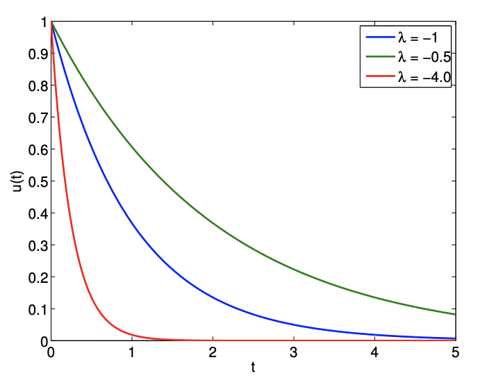
Note that solution starts from 1 (per the initial condition) and decays to zero for \(λ < 0\). The decay rate is controlled by the time constant \(1/|λ|\) — the larger the \(λ\), the faster the decay. The solution for a few different values of \(λ\) are shown in Figure 21.1. We note that for \(λ > 0\) the solution grows exponentially in time: the system is unstable. (In actual fact, in most physical situations, at some point additional terms — for example, nonlinear effects not included in our simple model — would become important and ensure saturation in some steady state.) In the remainder of this chapter unless specifically indicated otherwise we shall assume that \(λ < 0\).
Constant Forcing
Next, we consider a constant forcing case with \(u_0 = 0\) and \(f(t) = 1\), i.e.
\begin{aligned}
\frac{d u}{d t} &=\lambda u + 1, \\
u(0) &=0.
\end{aligned}
We have already found the homogeneous solution to the ODE. We now find the particular solution. Because the forcing term is constant, we consider a particular solution of the form \(u_p(t) = \gamma\). Substitution of \(u_p\) yields
\(0=\lambda \gamma+1 \quad \Rightarrow \quad \gamma=-\frac{1}{\lambda}\)
Thus, our solution is of the form
\(u(t) = − \frac{1} {λ} + \alpha e^{λt}\).
Enforcing the initial condition,
\(u(t=0)=-\frac{1}{\lambda}+\alpha=0 \quad \Rightarrow \quad \alpha=\frac{1}{\lambda}\)
Thus, our solution is given by
\(u(t) = \frac{1} {λ} (e^{λt} − 1) \).
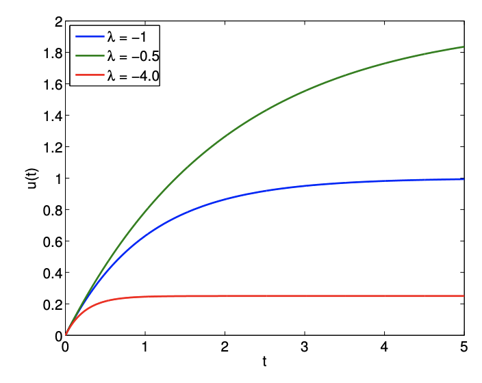
The solutions for a few different values of \(λ\) are shown in Figure 21.2. For \(λ < 0\), after the transient which decays on the time scale \(1/|λ|\), the solution settles to the steady state value of \(−1/λ\).
Sinusoidal Forcing
Let us consider a final case with \(u_0 = 0\) and a sinusoidal forcing, \(f(t) = cos(ωt)\), i.e.
\begin{aligned}
\frac{d u}{d t} &=\lambda u+\cos (\omega t) \\
u_{0} &=0
\end{aligned}
Because the forcing term is sinusoidal with the frequency \(ω\), the particular solution is of the form \(u_p(t) = \gamma sin(ωt) + δ cos(ωt)\). Substitution of the particular solution to the ODE yields
\begin{aligned}
(\mathrm{LHS}) &=\frac{d u_{p}}{d t}=\omega(\gamma \cos (\omega t)-\delta \sin (\omega t)) \\
(\mathrm{RHS}) &=\lambda(\gamma \sin (\omega t)+\delta \cos (\omega t))+\cos (\omega t)
\end{aligned}
Equating the LHS and RHS and collecting like coefficients we obtain
\(ω \gamma = λδ + 1 \),
\(−ωδ = λ\gamma\).
The solution to this linear system is given by \(\gamma = ω/(ω^2 + λ^2 )\) and \(δ = −λ/(ω^2 + λ^2 )\). Thus, the solution is of the form
\(u(t)=\frac{\omega}{\omega^{2}+\lambda^{2}} \sin (\omega t)-\frac{\lambda}{\omega^{2}+\lambda^{2}} \cos (\omega t)+\alpha e^{\lambda t}\)
Imposing the boundary condition, we obtain
\(u(t=0)=-\frac{\lambda}{\omega^{2}+\lambda^{2}}+\alpha=0 \quad \Rightarrow \quad \alpha=\frac{\lambda}{\omega^{2}+\lambda^{2}} .\)
Thus, the solution to the IVP with the sinusoidal forcing is
\(u(t)=\frac{\omega}{\omega^{2}+\lambda^{2}} \sin (\omega t)-\frac{\lambda}{\omega^{2}+\lambda^{2}}\left(\cos (\omega t)-e^{\lambda t}\right)\)
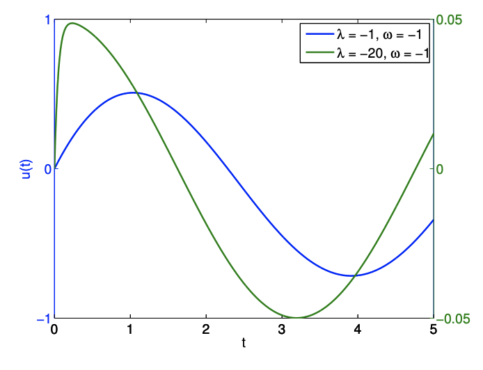
We note that for low frequency there is no phase shift; however, for high frequency there is a \(\pi/2\) phase shift.
The solutions for \(λ = −1, ω = 1\) and \(λ = −20, ω = 1\) are shown in Figure 21.3. The steady state behavior is controlled by the sinusoidal forcing function and has the time scale of \(1/ω\). On the other hand, the initial transient is controlled by \(λ\) and has the time scale of \(1/|λ|\). In particular, note that for \(|λ|>> ω\), the solution exhibits very different time scales in the transient and in the steady (periodic) state. This is an example of a stiff equation (we shall see another example at the conclusion of this unit). Solving a stiff equation introduces additional computational challenges for numerical schemes, as we will see shortly.
First Numerical Method: Euler Backward (Implicit)
In this section, we consider the Euler Backward integrator for solving initial value problems. We first introduce the time stepping scheme and then discuss a number of properties that characterize the scheme.
Discretization
In order to solve an IVP numerically, we first discretize the time domain \(]0, t_f ]\) into \(J\) segments. The discrete time points are given by
\(t^{j}=j \Delta t, \quad j=0,1, \ldots, J=t_{f} / \Delta t\)
where \(∆t\) is the time step. For simplicity, we assume in this chapter that the time step is constant throughout the time integration.
The Euler Backward method is obtained by applying the first-order Backward Difference Formula (see Unit I) to the time derivative. Namely, we approximate the time derivative by
\(\dfrac{du}{dt} \approx \dfrac{\tilde{u}^j - \tilde{u}{j-1}}{\Delta t}\),
where \(\tilde{u}^j = \tilde{u}(t^j )\) is the approximation to \(u(t^j )\) and \(∆t = t^j − t^{j−1}\) is the time step. Substituting the approximation into the differential equation, we obtain a difference equation
\(\dfrac{\tilde{u}^j - \tilde{u}^{j-1}}{\Delta t} = \lambda \tilde{u}^j + f(t^j), \quad j = 1,....,J\),
\(\tilde{u}^0 = u_0\),
for \(\tilde{u}^j, j = 0, . . . , J.\) Note the scheme is called “implicit” because time level \(j\) appears on the right-hand side. We can think of Euler Backward as a kind of rectangle, right integration rule — but now the integrand is not known a priori.
We anticipate that the solution \(\tilde{u}^j, j = 1, . . . , J,\) approaches the true solution \(u(t^j ), j = 1, . . . , J\), as the time step gets smaller and the finite difference approximation approaches the continuous system. In order for this convergence to the true solution to take place, the discretization must possess two important properties: consistency and stability. Note our analysis here is more subtle than the analysis in Unit I. In Unit I we looked at the error in the finite difference approximation; here, we are interested in the error induced by the finite difference approximation on the approximate solution of the ODE IVP.
Consistency
Consistency is a property of a discretization that ensures that the discrete equation approximates the same process as the underlying ODE as the time step goes to zero. This is an important property, because if the scheme is not consistent with the ODE, then the scheme is modeling a different process and the solution would not converge to the true solution.
Let us define the notion of consistency more formally. We first define the truncation error by substituting the true solution \(u(t)\) into the Euler Backward discretization, i.e.
\(τ_{\text{truc}}^j ≡ \dfrac{u(t^j) - u(t^{j-1})}{\Delta t} - \lambda u (t^j) - f(t^j), \quad j = 1,...,J\).
Note that the truncation error, \(τ^j_{\text{trunc}}\), measures the extent to which the exact solution to the ODE does not satisfy the difference equation. In general, the exact solution does not satisfy the difference equation, so \(τ^j_{\text{trunc}} \neq 0\). In fact, as we will see shortly, if \(τ^j_{\text{trunc}} = 0, j = 1, . . . , J\), then \(\tilde{u}^j = u(t^j ),\) i.e., \(\tilde{u}^j\) is the exact solution to the ODE at the time points.
We are particularly interested in the largest of the truncation errors, which is in a sense the largest discrepancy between the differential equation and the difference equation. We denote this using the infinity norm,
\(\left\|\tau_{\text {trunc }}\right\|_{\infty}=\max _{j=1, \ldots, J}\left|\tau_{\text {trunc }}^{j}\right|\)
A scheme is consistent with the ODE if
\(\left\|\tau_{\text {trunc }}\right\|_{\infty} \rightarrow 0 \quad \text { as } \quad \Delta t \rightarrow 0 \).
The difference equation for a consistent scheme approaches the differential equation as \(\Delta t \rightarrow\) 0 . However, this does not necessary imply that the solution to the difference equation, \(\tilde{u}\left(t^{j}\right)\), approaches the solution to the differential equation, \(u\left(t^{j}\right)\).
The Euler Backward scheme is consistent. In particular
\(\left\|\tau_{\text {trunc }}\right\|_{\infty} \leq \frac{\Delta t}{2} \max _{t \in\left[0, t_{f}\right]}\left|\frac{d^{2} u}{d t^{2}}(t)\right| \rightarrow 0 \quad \text { as } \quad \Delta t \rightarrow 0 .\)
We demonstrate this result below.
Begin Advanced Material
Let us now analyze the consistency of the Euler Backward integration scheme. We first apply Taylor expansion to \(u\left(t^{j-1}\right)\) about \(t^{j}\), i.e.
\(u\left(t^{j-1}\right)=u\left(t^{j}\right)-\Delta t \frac{d u}{d t}\left(t^{j}\right)-\underbrace{\int_{t^{j-1}}^{t^{j}}\left(\int_{t^{j-1}}^{\tau} \frac{d^{2} u}{d t^{2}}(\gamma) d \gamma\right) d \tau}_{s^{j}(u)} .\)
This result is simple to derive. By the fundamental theorem of calculus,
\(\int_{t^{j-1}}^{\tau} \frac{d u^{2}}{d t^{2}}(\gamma) d \gamma=\frac{d u}{d t}(\tau)-\frac{d u}{d t}\left(t^{j-1}\right) .\)
Integrating both sides over \(] t^{j-1}, t^{j}[\),
\begin{aligned}
\int_{t^{j-1}}^{t^{j}}\left(\int_{t^{j-1}}^{\tau} \frac{d u^{2}}{d t^{2}}(\gamma) d \gamma\right) d \tau &=\int_{t^{j-1}}^{t^{j}}\left(\frac{d u}{d t}(\tau)\right) d \tau-\int_{t^{j-1}}^{t^{j}}\left(\frac{d u}{d t}\left(t^{j-1}\right)\right) d \tau \\
&=u\left(t^{j}\right)-u\left(t^{j-1}\right)-\left(t^{j}-t^{j-1}\right) \frac{d u}{d t}\left(t^{j-1}\right) \\
&=u\left(t^{j}\right)-u\left(t^{j-1}\right)-\Delta t \frac{d u}{d t}\left(t^{j-1}\right)
\end{aligned}
Substitution of the expression to the right-hand side of the Taylor series expansion yields
\(u\left(t^{j}\right)-\Delta t \frac{d u}{d t}\left(t^{j}\right)-s^{j}(u)=u\left(t^{j}\right)-\Delta t \frac{d u}{d t}\left(t^{j}\right)-u\left(t^{j}\right)+u\left(t^{j-1}\right)+\Delta t \frac{d u}{d t}\left(t^{j-1}\right)=u\left(t^{j-1}\right),\)
which proves the desired result.
Substituting the Taylor expansion into the expression for the truncation error,
\begin{aligned}
\tau_{\text {trunc }}^{j} &=\frac{u\left(t^{j}\right)-u\left(t^{j-1}\right)}{\Delta t}-\lambda u\left(t^{j}\right)-f\left(t^{j}\right) \\
&=\frac{1}{\Delta t}\left(u\left(t^{j}\right)-\left(u\left(t^{j}\right)-\Delta t \frac{d u}{d t}\left(t^{j}\right)-s^{j}(u)\right)\right)-\lambda u\left(t^{j}\right)-f\left(t^{j}\right) \\
&=\underbrace{\frac{d u}{d t}\left(t^{j}\right)-\lambda u\left(t^{j}\right)-f\left(t^{j}\right)}_{=0: \text { by ODE }}+\frac{s^{j}(u)}{\Delta t} \\
&=\frac{s^{j}(u)}{\Delta t} .
\end{aligned}
We now bound the remainder term \(s^{j}(u)\) as a function of \(\Delta t\). Note that
\begin{aligned}
s^{j}(u) &=\int_{t^{j-1}}^{t^{j}}\left(\int_{t^{j-1}}^{\tau} \frac{d^{2} u}{d t^{2}}(\gamma) d \gamma\right) d \tau \leq \int_{t^{j-1}}^{t^{j}}\left(\int_{t^{j-1}}^{\tau}\left|\frac{d^{2} u}{d t^{2}}(\gamma)\right| d \gamma\right) d \tau \\
& \leq \max _{t \in\left[t^{j-1}, t^{j}\right]}\left|\frac{d^{2} u}{d t^{2}}(t)\right| \int_{t^{j-1}}^{t^{j}} \int_{t^{j-1}}^{\tau} d \gamma d \tau \\
&=\max _{t \in\left[t^{j-1}, t^{j}\right]}\left|\frac{d^{2} u}{d t^{2}}(t)\right| \frac{\Delta t^{2}}{2}, \quad j=1, \ldots, J .
\end{aligned}
So, the maximum truncation error is
\(\left\|\tau_{\text {trunc }}\right\|_{\infty}=\max _{j=1, \ldots, J}\left|\tau_{\text {trunc }}^{j}\right| \leq \max _{j=1, \ldots, J}\left(\frac{1}{\Delta t} \max _{t \in\left[t^{-1}, t, t^{j}\right]}\left|\frac{d^{2} u}{d t^{2}}(t)\right| \frac{\Delta t^{2}}{2}\right) \leq \frac{\Delta t}{2} \max _{t \in\left[0, t_{f}\right]}\left|\frac{d^{2} u}{d t^{2}}(t)\right|\)
We see that
\(\left\|\tau_{\text {trunc }}\right\|_{\infty} \leq \frac{\Delta t}{2} \max _{t \in\left[0, t_{f}\right]}\left|\frac{d^{2} u}{d t^{2}}(t)\right| \rightarrow 0 \quad \text { as } \quad \Delta t \rightarrow 0\)
Thus, the Euler Backward scheme is consistent.
Advanced Material
Stability
Stability is a property of a discretization that ensures that the error in the numerical approximation does not grow with time. This is an important property, because it ensures that a small truncation error introduced at each time step does not cause a catastrophic divergence in the solution over time.
To study stability, let us consider a homogeneous IVP,
\(\dfrac{du}{dt} = \lambda u\),
\(u(0) = 1\).
Recall that the true solution is of the form \(u(t) = e^{λt}\) and decays for \(λ < 0\). Applying the Euler Backward scheme, we obtain
\begin{aligned}
\frac{\tilde{u}^{j}-\tilde{u}^{j-1}}{\Delta t} &=\lambda \tilde{u}^{j}, \quad j=1, \ldots, J, \\
u^{0} &=1 .
\end{aligned}
A scheme is said to be absolutely stable if
\(\left|\tilde{u}^{j}\right| \leq\left|\tilde{u}^{j-1}\right|, \quad j=1, \ldots, J .\)
Alternatively, we can define the amplification factor, \(\gamma\), as
\(\gamma \equiv \frac{\left|\tilde{u}^{j}\right|}{\left|\tilde{u}^{j-1}\right|} .\)
Absolute stability requires that \(\gamma \leq 1\) for all \(j=1, \ldots, J\).
Let us now show that the Euler Backward scheme is stable for all \(\Delta t\) (for \(\lambda<0\) ). Rearranging the difference equation,
\begin{aligned}
\tilde{u}^{j}-\tilde{u}^{j-1} &=\lambda \Delta t \tilde{u}^{j} \\
\tilde{u}^{j}(1-\lambda \Delta t) &=\tilde{u}^{j-1} \\
\left|\tilde{u}^{j}\right||1-\lambda \Delta t| &=\left|\tilde{u}^{j-1}\right| .
\end{aligned}
So, we have
\(\gamma=\frac{\left|\tilde{u}^{j}\right|}{\left|\tilde{u}^{j-1}\right|}=\frac{1}{|1-\lambda \Delta t|} .\)
Recalling that \(\lambda<0\) (and \(\Delta t>0\) ), we have
\(\gamma=\frac{1}{1-\lambda \Delta t}<1 .\)
Thus, the Euler Backward scheme is stable for all $\Delta t$ for the model problem considered. The scheme is said to be unconditionally stable because it is stable for all \(\Delta t\). Some schemes are only conditionally stable, which means the scheme is stable for \(\Delta t \leq \Delta t_{\mathrm{cr}}\), where \(\Delta t_{\text {cr }}\) is some critical time step.
Convergence: Dahlquist Equivalence Theorem
Now we define the notion of convergence. A scheme is convergent if the numerical approximation approaches the analytical solution as the time step is reduced. Formally, this means that
\(\tilde{u}^{j} \equiv \tilde{u}\left(t^{j}\right) \rightarrow u\left(t^{j}\right) \quad\) for fixed \(t^{j}\) as \(\Delta t \rightarrow 0\)
Note that fixed time \(t^{j}\) means that the time index must go to infinity (i.e., an infinite number of time steps are required) as \(\Delta t \rightarrow 0\) because \(t^{j}=j \Delta t\). Thus, convergence requires that not too much error is accumulated at each time step. Furthermore, the error generated at a given step should not grow over time.
The relationship between consistency, stability, and convergence is summarized in the Dahlquist equivalence theorem. The theorem states that consistency and stability are the necessary and sufficient condition for a convergent scheme, i.e.
consistency \(+\) stability \(\Leftrightarrow\) convergence
Thus, we only need to show that a scheme is consistent and (absolutely) stable to show that the scheme is convergent. In particular, the Euler Backward scheme is convergent because it is consistent and (absolutely) stable.
Begin Advanced Material
Example 21.1.1 Consistency, stability, and convergence for Euler Backward
In this example, we will study in detail the relationship among consistency, stability, and convergence for the Euler Backward scheme. Let us denote the error in the solution by \(e^{j}\),
\(e^{j} \equiv u\left(t^{j}\right)-\tilde{u}\left(t^{j}\right)\)
We first relate the evolution of the error to the truncation error. To begin, we recall that
\begin{aligned}
&u\left(t^{j}\right)-u\left(t^{j-1}\right)-\lambda \Delta t u\left(t^{j}\right)-\Delta t f\left(t^{j}\right)=\Delta t \tau_{\text {trunc }}^{j} \\
&\tilde{u}\left(t^{j}\right)-\tilde{u}\left(t^{j-1}\right)-\lambda \Delta t \tilde{u}\left(t^{j}\right)-\Delta t f\left(t^{j}\right)=0
\end{aligned}
subtracting these two equations and using the definition of the error we obtain
\(e^{j}-e^{j-1}-\lambda \Delta t e^{j}=\Delta t \tau_{\text {trunc }}^{j}\)
or, rearranging the equation,
\((1-\lambda \Delta t) e^{j}-e^{j-1}=\Delta t \tau_{\text {trunc }}^{j}\).
We see that the error itself satisfies the Euler Backward difference equation with the truncation error as the source term. Clearly, if the truncation error \(τ^j_{\text{trunc}}\) is zero for all time steps (and initial error is zero), then the error remains zero. In other words, if the truncation error is zero then the scheme produces the exact solution at each time step.
However, in general, the truncation error is nonzero, and we would like to analyze its influence on the error. Let us multiply the equation by \((1 − λ∆t)^{j−1}\) to get
\((1-\lambda \Delta t)^{j} e^{j}-(1-\lambda \Delta t)^{j-1} e^{j-1}=(1-\lambda \Delta t)^{j-1} \Delta t \tau_{\text {trunc }}^{j}\)
Now, let us compute the sum for \(j=1, \ldots, n\), for some \(n \leq J\)
\(\sum_{j=1}^{n}\left[(1-\lambda \Delta t)^{j} e^{j}-(1-\lambda \Delta t)^{j-1} e^{j-1}\right]=\sum_{j=1}^{n}\left[(1-\lambda \Delta t)^{j-1} \Delta t \tau_{\text {trunc }}^{j}\right]\)
This is a telescopic series and all the middle terms on the left-hand side cancel. More explicitly,
\begin{aligned}
(1-\lambda \Delta t)^{n} e^{n}-(1-\lambda \Delta t)^{n-1} e^{n-1} &=(1-\lambda \Delta t)^{n-1} \Delta t \tau_{\text {trunc }}^{n} \\
(1-\lambda \Delta t)^{n-1} e^{n-1}-(1-\lambda \Delta t)^{n-2} e^{n-2} &=(1-\lambda \Delta t)^{n-2} \Delta t \tau_{\text {trunc }}^{n-1} \\
& \vdots \\
(1-\lambda \Delta t)^{2} e^{2}-(1-\lambda \Delta t)^{1} e^{1} &=(1-\lambda \Delta t)^{1} \Delta t \tau_{\text {trunc }}^{2} \\
(1-\lambda \Delta t)^{1} e^{1}-(1-\lambda \Delta t)^{0} e^{0} &=(1-\lambda \Delta t)^{0} \Delta t \tau_{\text {trunc }}^{1}
\end{aligned}
simplifies to
\((1-\lambda \Delta t)^{n} e^{n}-e^{0}=\sum_{j=1}^{n}(1-\lambda \Delta t)^{j-1} \Delta t \tau_{\text {trunc }}^{j}\)
Recall that we set \(\tilde{u}^{0}=\tilde{u}\left(t^{0}\right)=u\left(t^{0}\right)\), so the initial error is zero \(\left(e^{0}=0\right)\). Thus, we are left with
\((1-\lambda \Delta t)^{n} e^{n}=\sum_{j=1}^{n}(1-\lambda \Delta t)^{j-1} \Delta t \tau_{\text {trunc }}^{j}\)
or, equivalently,
\(e^{n}=\sum_{j=1}^{n}(1-\lambda \Delta t)^{j-n-1} \Delta t \tau_{\text {trunc }}^{j}\)
Recalling that \(\left\|\tau_{\text {trunc }}\right\|_{\infty}=\max _{j=1, \ldots, J}\left|\tau_{\text {trunc }}^{j}\right|\), we can bound the error by
\(\left|e^{n}\right| \leq \Delta t\left\|\tau_{\text {trunc }}\right\|_{\infty} \sum_{j=1}^{n}(1-\lambda \Delta t)^{j-n-1}\)
Recalling the amplification factor for the Euler Backward scheme, \(\gamma = 1/(1−λ∆t)\), the summation can be rewritten as
\begin{aligned}
\sum_{j=1}^{n}(1-\lambda \Delta t)^{j-n-1} &=\frac{1}{(1-\lambda \Delta t)^{n}}+\frac{1}{(1-\lambda \Delta t)^{n-1}}+\cdots+\frac{1}{(1-\lambda \Delta t)} \\
&=\gamma^{n}+\gamma^{n-1}+\cdots+\gamma .
\end{aligned}
Because the scheme is stable, the amplification factor satisfies \(\gamma \leq 1\). Thus, the sum is bounded by
\(\sum_{j=1}^{n}(1-\lambda \Delta t)^{j-n-1}=\gamma^{n}+\gamma^{n-1}+\cdots+\gamma \leq n \gamma \leq n\)
Thus, we have
\(\left|e^{n}\right| \leq(n \Delta t)\left\|\tau_{\text {trunc }}\right\|_{\infty}=t^{n}\left\|\tau_{\text {trunc }}\right\|_{\infty}\)
Furthermore, because the scheme is consistent, \(\left\|\tau_{\text {trunc }}\right\|_{\infty} \rightarrow 0\) as \(\Delta t \rightarrow 0\). Thus,
\(\left\|e^{n}\right\| \leq t^{n}\left\|\tau_{\text {trunc }}\right\|_{\infty} \rightarrow 0 \quad \text { as } \quad \Delta t \rightarrow 0\)
for fixed \(t^{n}=n \Delta t\). Note that the proof of convergence relies on stability \((\gamma \leq 1)\) and consistency \(\left(\left\|\tau_{\text {trunc }}\right\|_{\infty} \rightarrow 0\right.\) as \(\left.\Delta t \rightarrow 0\right)\).
Advanced Material
Order of Accuracy
The Dahlquist equivalence theorem shows that if a scheme is consistent and stable, then it is convergent. However, the theorem does not state how quickly the scheme converges to the true solution as the time step is reduced. Formally, a scheme is said to be \(p^{\rm th}\)-order accurate if
\(\left|e^{j}\right|<C \Delta t^{p} \quad \text { for a fixed } t^{j}=j \Delta t \text { as } \Delta t \rightarrow 0 .\)
The Euler Backward scheme is first-order accurate \((p=1)\), because
\(\left\|e^{j}\right\| \leq t^{j}\left\|\tau_{\text {trunc }}\right\|_{\infty} \leq t^{j} \frac{\Delta t}{2} \max _{t \in\left[0, t_{f}\right]}\left|\frac{d^{2} u}{d t^{2}}(t)\right| \leq C \Delta t^{1}\)
with
\(C=\frac{t_{f}}{2} \max _{t \in\left[0, t_{f}\right]}\left|\frac{d^{2} u}{d t^{2}}(t)\right|\)
(We use here \(t^{j} \leq t_{f}\).)
In general, for a stable scheme, if the truncation error is \(p^{\text {th }}\)-order accurate, then the scheme is \(p^{\text {th }}\)-order accurate, i.e.
\(\left\|\tau_{\text {trunc }}\right\|_{\infty} \leq C \Delta t^{p} \quad \Rightarrow \quad\left|e^{j}\right| \leq C \Delta t^{p} \quad \text { for a fixed } t^{j}=j \Delta t\)
In other words, once we prove the stability of a scheme, then we just need to analyze its truncation error to understand its convergence rate. This requires little more work than checking for consistency. It is significantly simpler than deriving the expression for the evolution of the error and analyzing the error behavior directly.
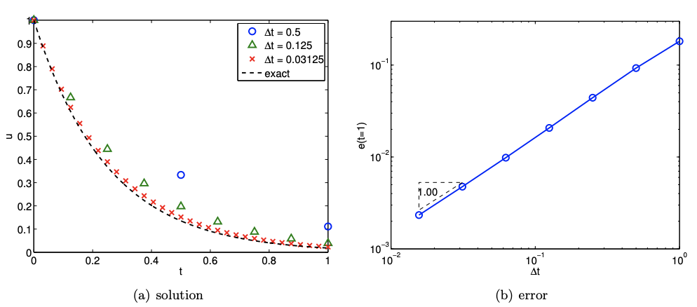
Figure 21.4 shows the error convergence behavior of the Euler Backward scheme applied to the homogeneous ODE with \(λ = −4\). The error is measured at \(t = 1\). Consistent with the theory, the scheme converges at the rate of \(p = 1\).
Explicit Scheme: Euler Forward
Let us now introduce a new scheme, the Euler Forward scheme. The Euler Forward scheme is obtained by applying the first-order forward difference formula to the time derivative, i.e.
\(\dfrac{du}{dt} \approx \dfrac{\tilde{u}^{j+1} - \tilde{u}^j}{\Delta t}\).
Substitution of the expression to the linear ODE yields a difference equation,
\begin{aligned}
\frac{\tilde{u}^{j+1}-\tilde{u}^{j}}{\Delta t} &=\lambda \tilde{u}^{j}+f\left(t^{j}\right), \quad j=0, \ldots, J-1 \\
\tilde{u}^{0} &=u_{0}
\end{aligned}
To maintain the same time index as the Euler Backward scheme (i.e., the difference equation involves the unknowns \(\tilde{u}^{j}\) and \(\tilde{u}^{j-1}\) ), let us shift the indices to obtain
\begin{aligned}
\frac{\tilde{u}^{j}-\tilde{u}^{j-1}}{\Delta t} &=\lambda \tilde{u}^{j-1}+f\left(t^{j-1}\right), \quad j=1, \ldots, J, \\
\tilde{u}^{0} &=u_{0} .
\end{aligned}
The key difference from the Euler Backward scheme is that the terms on the right-hand side are evaluated at \(t^{j-1}\) instead of at \(t^{j}\). Schemes for which the right-hand side does not involve time level \(j\) are known as "explicit" schemes. While the change may appear minor, this significantly modifies the stability. (It also changes the computational complexity, as we will discuss later.) We may view Euler Forward as a kind of "rectangle, left" integration rule.
Let us now analyze the consistency and stability of the scheme. The proof of consistency is similar to that for the Euler Backward scheme. The truncation error for the scheme is
\(\tau_{\text {trunc }}^{j}=\frac{u\left(t^{j}\right)-u\left(t^{j-1}\right)}{\Delta t}-\lambda u\left(t^{j-1}\right)-f\left(t^{j-1}\right) .\)
To analyze the convergence of the truncation error, we apply Taylor expansion to \(u\left(t^{j}\right)\) about \(t^{j-1}\) to obtain,
\(u\left(t^{j}\right)=u\left(t^{j-1}\right)+\Delta t \frac{d u}{d t}\left(t^{j-1}\right)+\underbrace{\int_{t^{j-1}}^{t^{j}}\left(\int_{t^{j-1}}^{\tau} \frac{d u^{2}}{d t^{2}}(\gamma) d \gamma\right) d \tau}_{s^{j}(u)}\)
Thus, the truncation error simplifies to
\begin{aligned}
\tau_{\text {trunc }}^{j} &=\frac{1}{\Delta t}\left(u\left(t^{j-1}\right)+\Delta t \frac{d u}{d t}\left(t^{j-1}\right)+s^{j}(u)-u\left(t^{j-1}\right)\right) \\
&=\underbrace{\frac{d u}{d t}\left(t^{j-1}\right)-\lambda u\left(t^{j-1}\right)-f\left(t^{j-1}\right)}_{=0: \text { by ODE }}+\frac{s^{j}(u)}{\Delta t} \\
&=\frac{s^{j}(u)}{\Delta t} .
\end{aligned}
In proving the consistency of the Euler Backward scheme, we have shown that \(s^{j}(u)\) is bounded by
\(s^{j}(u) \leq \max _{t \in\left[t^{j-1}, t^{j}\right]}\left|\frac{d^{2} u}{d t^{2}}(t)\right| \frac{\Delta t^{2}}{2}, \quad j=1, \ldots, J .\)
Thus, the maximum truncation error is bounded by
\(\left\|\tau_{\text {trunc }}\right\|_{\infty} \leq \max _{t \in\left[0, t_{f}\right]}\left|\frac{d^{2} u}{d t^{2}}(t)\right| \frac{\Delta t}{2} .\)
Again, the truncation error converges linearly with $\Delta t$ and the scheme is consistent because \(\left\|\tau_{\text {trunc }}\right\|_{\infty} \rightarrow 0\) as \(\Delta t \rightarrow 0\). Because the scheme is consistent, we only need to show that it is stable to ensure convergence.
To analyze the stability of the scheme, let us compute the amplification factor. Rearranging the difference equation for the homogeneous case,
\(\tilde{u}^{j}-\tilde{u}^{j-1}=\lambda \Delta t \tilde{u}^{j-1}\)
or
\(\left|\tilde{u}^{j}\right|=|1+\lambda \Delta t|\left|\tilde{u}^{j-1}\right|\)
which gives
\(\gamma=|1+\lambda \Delta t|\)
Thus, absolute stability (i.e., \(\gamma \leq 1\) ) requires
\begin{aligned}
&-1 \leq 1+\lambda \Delta t \leq 1 \\
&-2 \leq \lambda \Delta t \leq 0
\end{aligned}
Noting \(\lambda \Delta t \leq 0\) is a trivial condition for \(\lambda<0\), the condition for stability is
\(\Delta t \leq-\frac{2}{\lambda} \equiv \Delta t_{\mathrm{cr}}\)
Note that the Euler Forward scheme is stable only for \(\Delta t \leq 2 /|\lambda|\). Thus, the scheme is conditionally stable. Recalling the stability is a necessary condition for convergence, we conclude that the scheme converges for \(\Delta t \leq \Delta t_{\text {cr }}\), but diverges (i.e., blows up) with \(j\) if \(\Delta t>\Delta t_{\text {cr }}\).
Figure 21.5 shows the error convergence behavior of the Euler Forward scheme applied to the homogeneous ODE with \(\lambda=-4\). The error is measured at \(t=1\). The critical time step for stability is \(\Delta t_{\mathrm{cr}}=-2 / \lambda=1 / 2\). The error convergence plot shows that the error grows exponentially for
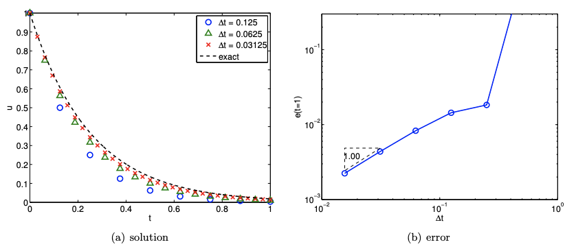
\(∆t > 1/2\). As \(∆t\) tends to zero, the numerical approximation converges to the exact solution, and the convergence rate (order) is \(p = 1\) — consistent with the theory. We should emphasize that the instability of the Euler Forward scheme for \(∆t > ∆t_{\rm cr}\) is not due to round-off errors and floating point representation (which involves “truncation,” but not truncation of the variety discussed in this chapter). In particular, all of our arguments for instability hold in infinite-precision arithmetic as well as finite-precision arithmetic. The instability derives from the difference equation; the instability amplifies truncation error, which is a property of the difference equation and differential equation. Of course, an unstable difference equation will also amplify round-off errors, but that is an additional consideration and not the main reason for the explosion in Figure 21.5.
Stiff Equations: Implicit vs. Explicit
Stiff equations are the class of equations that exhibit a wide range of time scales. For example, recall the linear ODE with a sinusoidal forcing,
\(\dfrac{du}{dt} = \lambda t + cos(ωt)\),
with \(|λ| >> ω\). The transient response of the solution is dictated by the time constant \(1/|λ|\). However, this initial transient decays exponentially with time. The long time response is governed by the time constant \(1/ω >> 1/|λ|\).
Let us consider the case with \(λ = −100\) and \(ω = 4\); the time scales differ by a factor of 25. The result of applying the Euler Backward and Euler Forward schemes with several different time steps is shown in Figure 21.6. Recall that the Euler Backward scheme is stable for any time step for \(λ < 0\). The numerical result confirms that the solution is bounded for all time steps considered. While a large time step (in particular \(∆t > 1/|λ|\)) results in an approximation which does not capture the initial transient, the long term behavior of the solution is still well represented. Thus, if the initial transient is not of interest, we can use a ∆t optimized to resolve only the long term behavior associated with the characteristic time scale of \(1/ω\) — in other words, \(∆t ∼ O(1/10)\),

rather than \(∆t ∼ O(1/|λ|)\). If \(|λ| >> ω\), then we significantly reduce the number of time steps (and thus the computational cost).
Unlike its implicit counterpart, the Euler Forward method is only conditionally stable. In particular, the critical time step for this problem is \(∆t_{\rm cr} = 2/|λ| = 0.02\). Thus, even if we are not interested in the initial transient, we cannot use a large time step because the scheme would be unstable. Only one of the three numerical solution (\(∆t = 1/64 < ∆t_{\rm cr}\)) is shown in Figure 21.6(c) because the other two time steps (\(∆t = 1/16, ∆t = 1/4\)) result in an unstable discretization and a useless approximation. The exponential growth of the error for \(∆t > ∆t_{\rm cr}\) is clearly reflected in Figure 21.6(d).
Stiff equations are ubiquitous in the science and engineering context; in fact, it is not uncommon to see scales that differ by over ten orders of magnitude. For example, the time scale associated with the dynamics of a passenger jet is several orders of magnitude larger than the time scale associated with turbulent eddies. If the dynamics of the smallest time scale is not of interest, then an unconditionally stable scheme that allows us to take arbitrarily large time steps may be computationally advantageous. In particular, we can select the time step that is necessary to achieve sufficient accuracy without any time step restriction arising from the stability consideration. Put another way, integration of a stiff system using a conditionally stable method may place a stringent requirement on the time step, rendering the integration prohibitively expensive. As none of the explicit schemes are unconditionally stable, implicit schemes are often preferred for stiff equations.
We might conclude from the above that explicit schemes serve very little purpose. In fact, this is not the case, because the story is a bit more complicated. In particular, we note that for Euler Backward, at every time step, we must effect a division operation, \(1/(1−(λ∆t))\), whereas for Euler Forward we must effect a multiplication, \(1 + (λ∆t)\). When we consider real problems of interest — systems, often large systems, of many and often nonlinear ODEs — these scalar algebraic operations of division for implicit schemes and multiplication for explicit schemes will translate into matrix inversion (more precisely, solution of matrix equations) and matrix multiplication, respectively. In general, and as we shall see in Unit V, matrix inversion is much more costly than matrix multiplication.
Hence the total cost equation is more nuanced. An implicit scheme will typically enjoy a larger time step and hence fewer time steps — but require more work for each time step (matrix solution). In contrast, an explicit scheme may require a much smaller time step and hence many more time steps — but will entail much less work for each time step. For stiff equations in which the \(∆t\) for accuracy is much, much larger than the \(∆t_{\rm cr}\) required for stability (of explicit schemes), typically implicit wins. On the other hand, for non-stiff equations, in which the \(∆t\) for accuracy might be on the same order as \(∆t_{\rm cr}\) required for stability (of explicit schemes), explicit can often win: in such cases we would in any event (for reasons of accuracy) choose a \(∆t \approx ∆t_{\rm cr}\); hence, since an explicit scheme will be stable for this \(∆t\), we might as well choose an explicit scheme to minimize the work per time step.
Unstable Equations
Absolute Stability and Stability Diagrams
We have learned that different integration schemes exhibit different stability characteristics. In particular, implicit methods tend to be more stable than explicit methods. To characterize the stability of different numerical integrators, let us introduce absolute stability diagrams. These diagrams allow us to quickly analyze whether an integration scheme will be stable for a given system.
Euler Backward
Let us construct the stability diagram for the Euler Backward scheme. We start with the homogeneous equation
\(\dfrac{dz}{dt} = \lambda z\).
So far, we have only considered a real \(λ\); now we allow \(λ\) to be a general complex number. (Later \(λ\) will represent an eigenvalue of a system, which in general will be a complex number.) The Euler
Backward discretization of the equation is
\(\frac{\tilde{z}^{j}-\tilde{z}^{j-1}}{\Delta t}=\lambda \tilde{z}^{j} \Rightarrow \quad \tilde{z}^{j}=(1-(\lambda \Delta t))^{-1} \tilde{z}^{j-1}\)
Recall that we defined the absolute stability as the region in which the amplification factor \(\gamma \equiv\) \(\left|\tilde{z}^{j}\right| /\left|\tilde{z}^{j-1}\right|\) is less than or equal to unity. This requires
\(\gamma=\frac{\left|\tilde{z}^{j}\right|}{\left|\tilde{z}^{j-1}\right|}=\left|\frac{1}{1-(\lambda \Delta t)}\right| \leq 1\)
We wish to find the values of \((\lambda \Delta t)\) for which the numerical solution exhibits a stable behavior (i.e., \(\gamma \leq 1\) ). A simple approach to achieve this is to solve for the stability boundary by setting the amplification factor to \(1=\left|e^{i \theta}\right|\), i.e.
\(e^{i \theta}=\frac{1}{1-(\lambda \Delta t)}\)
Solving for \((\lambda \Delta t)\), we obtain
\((\lambda \Delta t)=1-e^{-i \theta}\)
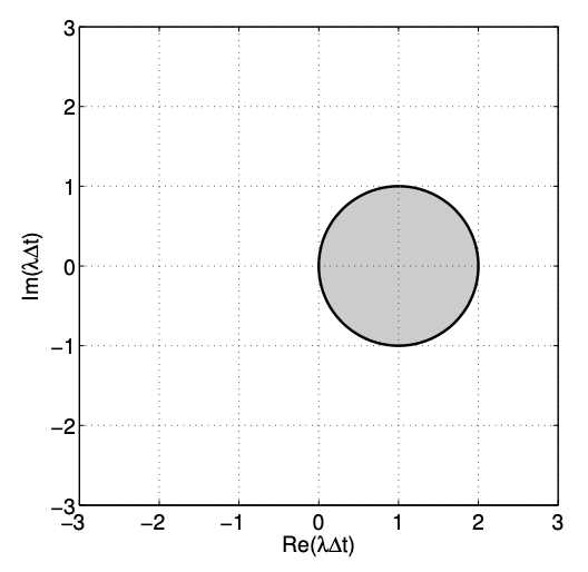
Thus, the stability boundary for the Euler Backward scheme is a circle of unit radius (the "one" multiplying \(e^{i \theta}\) ) centered at 1 (the one directly after the \(=\operatorname{sign}\) ).
To deduce on which side of the boundary the scheme is stable, we can check the amplification factor evaluated at a point not on the circle. For example, if we pick \(\lambda \Delta t=-1\), we observe that \(\gamma=1 / 2 \leq 1\). Thus, the scheme is stable outside of the unit circle. Figure 21.7 shows the stability diagram for the Euler Backward scheme. The scheme is unstable in the shaded region; it is stable in the unshaded region; it is neutrally stable, \(\left|\tilde{z}^{j}\right|=\left|\tilde{z}^{j-1}\right|\), on the unit circle. The unshaded region \((\gamma<1)\) and the boundary of the shaded and unshaded regions \((\gamma=1)\) represent the absolute stability region; the entire picture is denoted the absolute stability diagram.
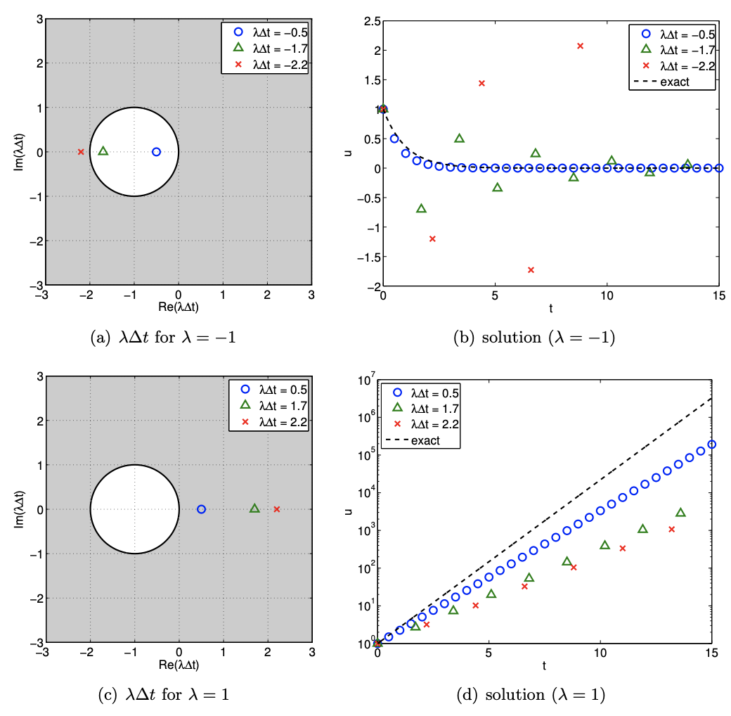
To gain understanding of the stability diagram, let us consider the behavior of the Euler Backward scheme for a few select values of \(\lambda \Delta t\). First, we consider a stable homogeneous equation, with \(\lambda=-1<0\). We consider three different values of \(\lambda \Delta t,-0.5,-1.7\), and \(-2.2\). Figure 21.8 (a) shows

the three points on the stability diagram that correspond to these choices of \(λ∆t\). All three points lie in the unshaded region, which is a stable region. Figure 21.8(b) shows that all three numerical solutions decay with time as expected. While the smaller \(∆t\) results in a smaller error, all schemes are stable and converge to the same steady state solution.
Begin Advanced Material
Next, we consider an unstable homogeneous equation, with \(λ = 1 > 0\). We again consider three different values of \(λ∆t, 0.5, 1.7\), and \(2.2.\) Figure 21.8(c) shows that two of these points lie in the unstable region, while \(λ∆t = 2.2\) lies in the stable region. Figure 21.8(d) confirms that the solutions for \(λ∆t = 0.5\) and \(1.7\) grow with time, while \(λ∆t = 2.2\) results in a decaying solution. The true solution, of course, grows exponentially with time. Thus, if the time step is too large (specifically \(λ∆t > 2\)), then the Euler Backward scheme can produce a decaying solution even if the true solution grows with time — which is undesirable; nevertheless, as \(∆t \rightarrow 0\), we obtain the correct behavior. In general, the interior of the absolute stability region should not include \(λ∆t = 0\). (In fact \(λ∆t = 0\) should be on the stability boundary.)
Advanced Material
Euler Forward
Let us now analyze the absolute stability characteristics of the Euler Forward scheme. Similar to the Euler Backward scheme, we start with the homogeneous equation. The Euler Forward discretization of the equation yields
\(\dfrac{\tilde{z}^j - \tilde{z}^{j-1}}{\Delta t} = \lambda \tilde{z}^{j-1} \Rightarrow \tilde{z}^j = \left ( 1 + (\lambda \Delta t) \right) \tilde{z}^{j-1}\).
The stability boundary, on which the amplification factor is unity, is given by
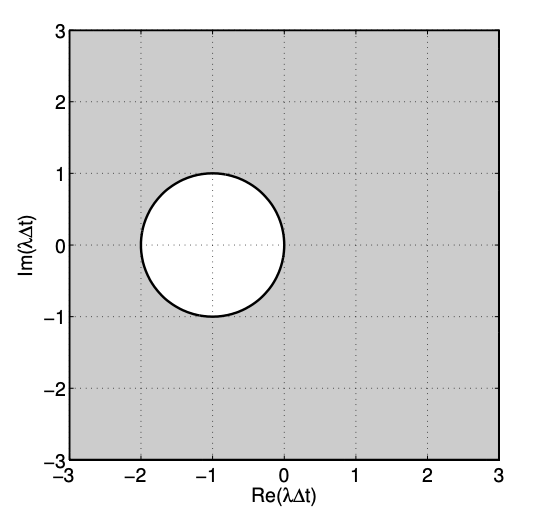
\(\gamma = |1 + (\lambda \Delta t)| = 1 \Rightarrow (\lambda \Delta t) = e^{-i \Theta} - 1\)
The stability boundary is a circle of unit radius centered at \(−1\). Substitution of, for example, \(λ∆t = −1/2\), yields \(\gamma(λ∆t = −1/2) = 1/2\), so the amplification is less than unity inside the circle. The stability diagram for the Euler Forward scheme is shown in Figure 21.9.
As in the Euler Backward case, let us pick a few select values of λ∆t and study the behavior of the Euler Forward scheme. The stability diagram and solution behavior for a stable ODE (\(λ = −1 < 0\)) are shown in Figure 21.10(a) and 21.10(b), respectively. The cases with \(λ∆t = −0.5\) and \(−1.7\) lie in the stable region of the stability diagram, while \(λ∆t = −2.2\) lies in the unstable region. Due to instability, the numerical solution for \(λ∆t = −2.2\) diverges exponentially with time, even though the true solution decays with time. The solution for \(λ∆t = −1.7\) shows some oscillation, but the magnitude of the oscillation decays with time, agreeing with the stability diagram. (For an unstable ODE (\(λ = 1 > 0\)), Figure 21.10(c) shows that all time steps considered lie in the unstable region of the stability diagram. Figure 21.10(d) confirms that all these choices of ∆t produce a growing solution.)
Multistep Schemes
We have so far considered two schemes: the Euler Backward scheme and the Euler Forward scheme. These two schemes compute the state \(\tilde{u}^j\) from the previous state \(\tilde{u}^{j−1}\) and the source function
evaluated at \(t^j\) or \(t^{j−1}\). The two schemes are special cases of multistep schemes, where the solution at the current time \(\tilde{u}^j\) is approximated from the previous solutions. In general, for an ODE of the form
\(\dfrac{du}{dt} = g(u,t)\),
a \(K\)-step multistep scheme takes the form
\begin{aligned}
\sum_{k=0}^{K} \alpha_{k} \tilde{u}^{j-k} &=\Delta t \sum_{k=0}^{K} \beta_{k} g^{j-k}, \quad j=1 \\
\tilde{u}^{j} &=u_{0}
\end{aligned}
where \(g^{j-k}=g\left(\tilde{u}^{j-k}, t^{j-k}\right)\). Note that the linear ODE we have been considering results from the choice \(g(u, t)=\lambda u+f(t)\). A \(K\)-step multistep scheme requires solutions (and derivatives) at \(K\) previous time steps. Without loss of generality, we choose \(\alpha_{0}=1\). A scheme is uniquely defined by choosing \(2 K+1\) coefficients, \(\alpha_{k}, k=1, \ldots, K\), and \(\beta_{k}, k=0, \ldots, K\).
Multistep schemes can be categorized into implicit and explicit schemes. If we choose \(\beta_{0}=0\), then \(\tilde{u}^{j}\) does not appear on the right-hand side, resulting in an explicit scheme. As discussed before, explicit schemes are only conditionally stable, but are computationally less expensive per step. If we choose \(\beta_{0} \neq 0\), then \(\tilde{u}^{j}\) appears on the right-hand side, resulting in an implicit scheme. Implicit schemes tend to be more stable, but are more computationally expensive per step, especially for a system of nonlinear ODEs.
Let us recast the Euler Backward and Euler Forward schemes in the multistep method framework.
Example 21.1.2 Euler Backward as a multistep scheme
The Euler Backward scheme is a 1-step method with the choices
\(\alpha_{1}=-1, \quad \beta_{0}=1, \quad \text { and } \quad \beta_{1}=0 .\)
This results in
\(\tilde{u}^{j}-\tilde{u}^{j-1}=\Delta t g^{j}, \quad j=1, \ldots, J\)
______________________.______________________
Example 21.1.3 Euler Forward as a multistep scheme
The Euler Forward scheme is a 1-step method with the choices
\(\alpha_{1}=-1, \quad \beta_{0}=0, \quad \text { and } \quad \beta_{1}=1 .\)
This results in
\(\tilde{u}^{j}-\tilde{u}^{j-1}=\Delta t g^{j-1}, \quad j=1, \ldots, J\)
______________________.______________________
Now we consider three families of multistep schemes: Adams-Bashforth, Adams-Moulton, and Backward Differentiation Formulas.
Adams-Bashforth Schemes
Adams-Bashforth schemes are explicit multistep time integration schemes \(\left(\beta_{0}=0\right)\). Furthermore, we restrict ourselves to
\(\alpha_{1}=-1 \quad \text { and } \quad \alpha_{k}=0, \quad k=2, \ldots, K .\)
The resulting family of the schemes takes the form
\(\tilde{u}^{j}=\tilde{u}^{j-1}+\sum_{k=1}^{K} \beta_{k} g^{j-k}\)
Now we must choose \(\beta_{k}, k=1, \ldots K\), to define a scheme. To choose the appropriate values of \(\beta_{k}\), we first note that the true solution \(u\left(t^{j}\right)\) and \(u\left(t^{j-1}\right)\) are related by
\[u\left(t^{j}\right)=u\left(t^{j-1}\right)+\int_{t^{j-1}}^{t^{j}} \frac{d u}{d t}(\tau) d \tau=u\left(t^{j-1}\right)+\int_{t^{j-1}}^{t^{j}} g(u(\tau), \tau) d \tau . \tag{21.1} \]
Then, we approximate the integrand \(g(u(\tau), \tau), \tau \in\left(t^{j-1}, t^{j}\right)\), using the values \(g^{j-k}, k=1, \ldots, K\). Specifically, we construct a \((K-1)^{\text {th }}\)-degree polynomial \(p(\tau)\) using the \(K\) data points, i.e.
\(p(\tau)=\sum_{k=1}^{K} \phi_{k}(\tau) g^{j-k}\),
where \(\phi_{k}(\tau), k=1, \ldots, K\), are the Lagrange interpolation polynomials defined by the points \(t^{j-k}, k=1, \ldots, K\). Recalling the polynomial interpolation theory from Unit I, we note that the \((K-1)^{\text {th }}\)-degree polynomial interpolant is \(K^{\text {th }}\)-order accurate for \(g(u(\tau), \tau)\) sufficiently smooth, i.e.
\(p(\tau)=g(u(\tau), \tau)+\mathcal{O}\left(\Delta t^{K}\right) .\)
(Note in fact here we consider "extrapolation" of our interpolant.) Thus, we expect the order of approximation to improve as we incorporate more points given sufficient smoothness. Substitution of the polynomial approximation of the derivative to Eq. (21.1) yields
\(u\left(t^{j}\right) \approx u\left(t^{j-1}\right)+\int_{t^{j-1}}^{t^{j}} \sum_{k=1}^{K} \phi_{k}(\tau) g^{j-k} d \tau=u\left(t^{j-1}\right)+\sum_{k=1}^{K} \int_{t^{j-1}}^{t^{j}} \phi_{k}(\tau) d \tau g^{j-k} .\)
To simplify the integral, let us consider the change of variable \(\tau=t^{j}-\left(t^{j}-t^{j-1}\right) \hat{\tau}=t^{j}-\Delta t \hat{\tau}\). The change of variable yields
\(u\left(t^{j}\right) \approx u\left(t^{j-1}\right)+\Delta t \sum_{k=1}^{K} \int_{0}^{1} \hat{\phi}_{k}(\hat{\tau}) d \hat{\tau} g^{j-k}\)
where the \(\hat{\phi}_{k}\) are the Lagrange polynomials associated with the interpolation points \(\hat{\tau}=1,2, \ldots, K\). We recognize that the approximation fits the Adams-Bashforth form if we choose
\(\beta_{k}=\int_{0}^{1} \hat{\phi}_{k}(\hat{\tau}) d \hat{\tau} \).
Let us develop a few examples of Adams-Bashforth schemes.
Example 21.1.4 1-step Adams-Bashforth (Euler Forward)
The 1-step Adams-Bashforth scheme requires evaluation of \(\beta_{1}\). The Lagrange polynomial for this case is a constant polynomial, \(\hat{\phi}_{1}(\hat{\tau})=1\). Thus, we obtain
\(\beta_{1}=\int_{0}^{1} \hat{\phi}_{1}(\hat{\tau}) d \hat{\tau}=\int_{0}^{1} 1 d \hat{\tau}=1\).
Thus, the scheme is
\(\tilde{u}^j = \tilde{u}^{j-1} + \Delta t g^{j-1}\),
which is the Euler Forward scheme, first-order accurate.
______________________.______________________
Example 21.1.5 2-step Adams-Bashforth
The 2-step Adams-Bashforth scheme requires specification of \(\beta_1\) and \(\beta_2\). The Lagrange interpolation polynomials for this case are linear polynomials
\(\hat{\phi}_{1}(\hat{\tau})=-\hat{\tau}+2 \quad$ and $\quad \hat{\phi}_{2}(\hat{\tau})=\hat{\tau}-1\)
It is easy to verify that these are the Lagrange polynomials because \(\hat{\phi}_{1}(1)=\hat{\phi}_{2}(2)=1\) and \(\hat{\phi}_{1}(2)=\hat{\phi}_{2}(1)=0\). Integrating the polynomials
\begin{aligned}
&\beta_{1}=\int_{0}^{1} \phi_{1}(\hat{\tau}) d \hat{\tau}=\int_{0}^{1}(-\hat{\tau}+2) d \hat{\tau}=\frac{3}{2}, \\
&\beta_{2}=\int_{0}^{1} \phi_{2}(\hat{\tau}) d \hat{\tau}=\int_{0}^{1}(\hat{\tau}-1) d \hat{\tau}=-\frac{1}{2}
\end{aligned}
The resulting scheme is
\(\tilde{u}^{j}=\tilde{u}^{j-1}+\Delta t\left(\frac{3}{2} g^{j-1}-\frac{1}{2} g^{j-2}\right) .\)
This scheme is second-order accurate.
______________________.______________________
Adams-Moulton Schemes
Adams-Moulton schemes are implicit multistep time integration schemes \(\left(\beta_{0} \neq 0\right)\). Similar to Adams-Bashforth schemes, we restrict ourselves to
\(\alpha_{1}=-1 \quad \text { and } \quad \alpha_{k}=0, \quad k=2, \ldots, K .\)
The Adams-Moulton family of the schemes takes the form
\(\tilde{u}^{j}=\tilde{u}^{j-1}+\sum_{k=0}^{K} \beta_{k} g^{j-k}\)
We must choose \(\beta_{k}, k=1, \ldots, K\) to define a scheme. The choice of \(\beta_{k}\) follows exactly the same procedure as that for Adams-Bashforth. Namely, we consider the expansion of the form Eq. (21.1) and approximate \(g(u(\tau), \tau)\) by a polynomial. This time, we have \(K+1\) points, thus we construct a \(K^{\text {th }}\)-degree polynomial
\(p(\tau)=\sum_{k=0}^{K} \phi_{k}(\tau) g^{j-k},\)
where \(\phi_{k}(\tau), k=0, \ldots, K\), are the Lagrange interpolation polynomials defined by the points \(t^{j-k}\), \(k=0, \ldots, K\). Note that these polynomials are different from those for the Adams-Bashforth schemes due to the inclusion of \(t^{j}\) as one of the interpolation points. (Hence here we consider true interpolation, not extrapolation.) Moreover, the interpolation is now \((K+1)^{\text {th }}\)-order accurate.
Using the same change of variable as for Adams-Bashforth schemes, \(\tau=t^{j}-\Delta t \hat{\tau}\), we arrive at a similar expression,
\(u\left(t^{j}\right) \approx u\left(t^{j-1}\right)+\Delta t \sum_{k=0}^{K} \int_{0}^{1} \hat{\phi}_{k}(\hat{\tau}) d \hat{\tau} g^{j-k}\)
for the Adams-Moulton schemes; here the \(\hat{\phi}_{k}\) are the \(K^{\text {th }}\)-degree Lagrange polynomials defined by the points \(\hat{\tau}=0,1, \ldots, K\). Thus, the \(\beta_{k}\) are given by
\(\beta_{k}=\int_{0}^{1} \hat{\phi}_{k}(\hat{\tau}) d \hat{\tau} .\)
Let us develop a few examples of Adams-Moulton schemes.
Example 21.1.6 0-step Adams-Moulton (Euler Backward)
The 0-step Adams-Moulton scheme requires just one coefficient, \(\beta_{0}\). The "Lagrange" polynomial is \(0^{\text {th }}\) degree, i.e. a constant function \(\hat{\phi}_{0}(\hat{\tau})=1\), and the integration of the constant function over the unit interval yields
\(\beta_{0}=\int_{0}^{1} \hat{\phi}_{0}(\hat{\tau}) d \hat{\tau}=\int_{0}^{1} 1 d \hat{\tau}=1 .\)
Thus, the 0-step Adams-Moulton scheme is given by
\(\tilde{u}^{j}=\tilde{u}^{j-1}+\Delta t g^{j},\)
which in fact is the Euler Backward scheme. Recall that the Euler Backward scheme is first-order accurate.
______________________.______________________
Example 21.1.7 1-step Adams-Moulton (Crank-Nicolson)
The 1-step Adams-Moulton scheme requires determination of two coefficients, \(\beta_0\) and \(\beta_1\). The Lagrange polynomials for this case are linear polynomials
\(\hat{\phi}_{0}(\hat{\tau})=-\tau+1 \quad$ and $\quad \hat{\phi}_{1}(\hat{\tau})=\tau\)
Integrating the polynomials,
\begin{aligned}
&\beta_{0}=\int_{0}^{1} \hat{\phi}_{0}(\hat{\tau}) d \hat{\tau}=\int_{0}^{1}(-\tau+1) d \hat{\tau}=\frac{1}{2} \\
&\beta_{1}=\int_{0}^{1} \hat{\phi}_{1}(\hat{\tau}) d \hat{\tau}=\int_{0}^{1} \hat{\tau} d \hat{\tau}=\frac{1}{2}
\end{aligned}
The choice of \(\beta_{k}\) yields the Crank-Nicolson scheme
\(\tilde{u}^{j}=\tilde{u}^{j-1}+\Delta t\left(\frac{1}{2} g^{j}+\frac{1}{2} g^{j-1}\right)\).
The Crank-Nicolson scheme is second-order accurate. We can view Crank-Nicolson as a kind of "trapezoidal" rule.
______________________.______________________
Example 21.1.8 2-step Adams-Moulton
The 2-step Adams-Moulton scheme requires three coefficients, \(\beta_{0}, \beta_{1}\), and \(\beta_{2}\). The Lagrange polynomials for this case are the quadratic polynomials
\begin{aligned}
&\hat{\phi}_{0}(\hat{\tau})=\frac{1}{2}(\hat{\tau}-1)(\hat{\tau}-2)=\frac{1}{2}\left(\hat{\tau}^{2}-3 \hat{\tau}\right. \\
&\hat{\phi}_{1}(\hat{\tau})=-\hat{\tau}(\hat{\tau}-2)=-\hat{\tau}^{2}+2 \hat{\tau} \\
&\hat{\phi}_{2}(\hat{\tau})=\frac{1}{2} \hat{\tau}(\hat{\tau}-1)=\frac{1}{2}\left(\hat{\tau}^{2}-\hat{\tau}\right)
\end{aligned}
Integrating the polynomials,
\begin{aligned}
&\beta_{0}=\int_{0}^{1} \hat{\phi}_{0}(\hat{\tau}) d \hat{\tau}=\int_{0}^{1} \frac{1}{2}\left(\hat{\tau}^{2}-3 \hat{\tau}+2\right) \hat{\tau}=\frac{5}{12} \\
&\beta_{1}=\int_{0}^{1} \hat{\phi}_{1}(\hat{\tau}) d \hat{\tau}=\int_{0}^{1}\left(-\hat{\tau}^{2}+2 \hat{\tau}\right) d \hat{\tau}=\frac{2}{3} \\
&\beta_{2}=\int_{0}^{1} \hat{\phi}_{2}(\hat{\tau}) d \hat{\tau}=\int_{0}^{1} \frac{1}{2}\left(\hat{\tau}^{2}-\hat{\tau}\right) d \hat{\tau}=-\frac{1}{12}
\end{aligned}
Thus, the 2-step Adams-Moulton scheme is given by
\(\tilde{u}^{j}=\tilde{u}^{j-1}+\Delta t\left(\frac{5}{12} g^{j}+\frac{2}{3} g^{j-1}-\frac{1}{12} g^{j-2}\right)\).
This AM2 scheme is third-order accurate.
______________________.______________________
Convergence of Multistep Schemes: Consistency and Stability
Let us now introduce techniques for analyzing the convergence of a multistep scheme. Due to the Dahlquist equivalence theorem, we only need to show that the scheme is consistent and stable.
To show that the scheme is consistent, we need to compute the truncation error. Recalling that the local truncation error is obtained by substituting the exact solution to the difference equation (normalized such that \(\tilde{u}^{j}\) has the coefficient of 1 ) and dividing by \(\Delta t\), we have for any multistep schemes
\(\tau_{\text {trunc }}^{j}=\frac{1}{\Delta t}\left[u\left(t^{j}\right)+\sum_{k=1}^{K} \alpha_{k} u\left(t^{j-k}\right)\right]-\sum_{k=0}^{K} \beta_{k} g\left(t^{j-k}, u\left(t^{j-k}\right)\right)\).
For simplicity we specialize our analysis to the Adams-Bashforth family, such that
\(\tau_{\text {trunc }}^{j}=\frac{1}{\Delta t}\left(u\left(t^{j}\right)-u\left(t^{j-1}\right)\right)-\sum_{k=1}^{n} \beta_{k} g\left(t^{j-k}, u\left(t^{j-k}\right)\right)\).
We recall that the coefficients \(\beta_{k}\) were selected to match the extrapolation from polynomial fitting. Backtracking the derivation, we simplify the sum as follows
\begin{aligned}
\sum_{k=1}^{K} \beta_{k} g\left(t^{j-k}, u\left(t^{j-k}\right)\right) &=\sum_{k=1}^{K} \int_{0}^{1} \hat{\phi}_{k}(\hat{\tau}) d \hat{\tau} g\left(t^{j-k}, u\left(t^{j-k}\right)\right) \\
&=\sum_{k=1}^{K} \frac{1}{\Delta t} \int_{t^{j-1}}^{t^{j}} \phi_{k}(\tau) d \tau g\left(t^{j-k}, u\left(t^{j-k}\right)\right) \\
&=\frac{1}{\Delta t} \int_{t^{j-1}}^{t^{j}}\left[\sum_{k=1}^{K} \phi_{k}(\tau) g\left(t^{j-k}, u\left(t^{j-k}\right)\right)\right] d \tau \\
&=\frac{1}{\Delta t} \int_{t^{j-1}}^{t^{j}} p(\tau) d \tau
\end{aligned}
We recall that \(p(\tau)\) is a \((K-1)^{\text {th }}\)-degree polynomial approximating \(g(\tau, u(\tau))\). In particular, it is a \(K^{\text {th }}\)-order accurate interpolation with the error \(\mathcal{O}\left(\Delta t^{K}\right)\). Thus,
\begin{aligned}
\tau_{\text {trunc }}^{j} &=\frac{1}{\Delta t}\left(u\left(t^{j}\right)-u\left(t^{j-1}\right)\right)-\sum_{k=1}^{K} \beta_{k} g\left(t^{j-k}, u\left(t^{j-k}\right)\right) \\
&=\frac{1}{\Delta t}\left(u\left(t^{j}\right)-u\left(t^{j-1}\right)\right)-\frac{1}{\Delta t} \int_{t^{j-1}}^{t^{j}} g(\tau, u(\tau)) d \tau+\frac{1}{\Delta t} \int_{j^{j-1}}^{t^{j}} \mathcal{O}\left(\Delta t^{K}\right) d \tau \\
&=\frac{1}{\Delta t}\left[u\left(t^{j}\right)-u\left(t^{j-1}\right)-\int_{t^{j-1}}^{t^{j}} g(\tau, u(\tau)) d \tau\right]+\mathcal{O}\left(\Delta t^{K}\right) \\
&=\mathcal{O}\left(\Delta t^{K}\right) .
\end{aligned}
Note that the term in the bracket vanishes from \(g=d u / d t\) and the fundamental theorem of calculus. The truncation error of the scheme is \(\mathcal{O}\left(\Delta t^{K}\right)\). In particular, since \(K>0\), \(\tau_{\text {trunc }} \rightarrow 0\) as \(\Delta t \rightarrow 0\) and the Adams-Bashforth schemes are consistent. Thus, if the schemes are stable, they would converge at \(\Delta t^{K}\).
The analysis of stability relies on a solution technique for difference equations. We first restrict ourselves to linear equation of the form \(g(t, u)=\lambda u\). By rearranging the form of difference equation for the multistep methods, we obtain
\(\sum_{k=0}^{K}\left(\alpha_{k}-(\lambda \Delta t) \beta_{k}\right) \tilde{u}^{j-k}=0, \quad j=1, \ldots, J\)
The solution to the difference equation is governed by the initial condition and the \(K\) roots of the polynomial
\(q(x)=\sum_{k=0}^{K}\left(\alpha_{k}-(\lambda \Delta t) \beta_{k}\right) x^{K-k}\).
In particular, for any initial condition, the solution will exhibit a stable behavior if all roots \(r_{k}\), \(k=1, \ldots, K\), have magnitude less than or equal to unity. Thus, the absolute stability condition for multistep schemes is
\((\lambda \Delta t)\) such that \(\left|r_{K}\right| \leq 1, \quad k=1, \ldots, K\)
where \(r_{k}, k=1, \ldots, K\) are the roots of \(q\).
Example 21.1.9 Stability of the 2-step Adams-Bashforth scheme
Recall that the 2-step Adams-Bashforth results from the choice
\(\alpha_{0}=1, \quad \alpha_{1}=-1, \quad \alpha_{2}=0, \quad \beta_{0}=0, \quad \beta_{1}=\frac{3}{2}, \quad \text { and } \quad \beta_{2}=-\frac{1}{2}\).
The stability of the scheme is governed by the roots of the polynomial
\(q(x)=\sum_{k=0}^{2}\left(\alpha_{k}-(\lambda \Delta t) \beta_{k}\right) x^{2-k}=x^{2}+\left(-1-\frac{3}{2}(\lambda \Delta t)\right) x+\frac{1}{2}(\lambda \Delta t)=0\).
The roots of the polynomial are given by
\(r_{1,2}=\frac{1}{2}\left[1+\frac{3}{2}(\lambda \Delta t) \pm \sqrt{\left(1+\frac{3}{2}(\lambda \Delta t)\right)^{2}-2(\lambda \Delta t)}\right]\).
We now look for \((\lambda \Delta t)\) such that \(\left|r_{1}\right| \leq 1\) and \(\left|r_{2}\right| \leq 1\).
It is a simple matter to determine if a particular \(\lambda \Delta t\) is inside, on the boundary of, or outside the absolute stability region. For example, for \(\lambda \Delta t=-1\) we obtain \(r_{1}=-1, r_{2}=1 / 2\) and hence since \(\left|r_{1}\right|=1-\lambda \Delta t=-1\) is in fact on the boundary of the absolute stability diagram. Similarly, it is simple to confirm that \(\lambda \Delta t=-1 / 2\) yields both \(r_{1}\) and \(r_{2}\) of modulus strictly less than 1, and hence \(\lambda \Delta t=-1 / 2\) is inside the absolute stability region. We can thus in principle check each point \(\lambda \Delta t\) (or enlist more sophisticated solution procedures) in order to construct the full absolute stability diagram.
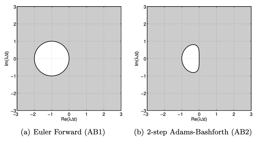
We shall primarily be concerned with the use of the stability diagram rather than the construction of the stability diagram - which for most schemes of interest are already derived and well documented. We present in Figure 21.11(b) the absolute stability diagram for the 2-step AdamsBashforth scheme. For comparison we show in Figure 21.11(a) the absolute stability diagram for Euler Forward, which is the 1-step Adams-Bashforth scheme. Note that the stability region of the Adams-Bashforth schemes are quite small; in fact the stability region decreases further for higher order Adams-Bashforth schemes. Thus, the method is only well suited for non-stiff equations.
______________________.______________________
Example 21.1.10 Stability of the Crank-Nicolson scheme
Let us analyze the absolute stability of the Crank-Nicolson scheme. Recall that the stability of a multistep scheme is governed by the roots of the polynomial
\(q(x)=\sum_{k=0}^{K}\left(\alpha_{k}-\lambda \Delta t \beta_{k}\right) x^{K-k}\).
For the Crank-Nicolson scheme, we have \(\alpha_{0}=1, \alpha_{1}=-1, \beta_{0}=1 / 2\), and \(\beta_{1}=1 / 2\). Thus, the polynomial is
\(q(x)=\left(1-\frac{1}{2}(\lambda \Delta t)\right) x+\left(-1-\frac{1}{2}(\lambda \Delta t)\right)\).
The root of the polynomial is
\(r=\frac{2+(\lambda \Delta t)}{2-(\lambda \Delta t)}\).
To solve for the stability boundary, let us set \(|r|=1=\left|e^{i \theta}\right|\) and solve for \((\lambda \Delta t)\), i.e.
\(\frac{2+(\lambda \Delta t)}{2-(\lambda \Delta t)}=e^{i \theta} \quad \Rightarrow \quad(\lambda \Delta t)=\frac{2\left(e^{i \theta}-1\right)}{e^{i \theta}+1}=\frac{i 2 \sin (\theta)}{1+\cos (\theta)}\).
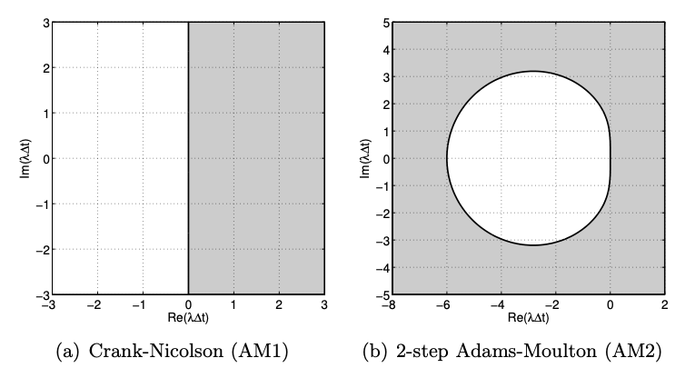
Thus, as \(\theta\) varies from 0 to \(\pi / 2, \lambda \Delta t\) varies from 0 to \(i \infty\) along the imaginary axis. Similarly, as \(\theta\) varies from 0 to \(-\pi / 2, \lambda \Delta t\) varies from 0 to \(-i \infty\) along the imaginary axis. Thus, the stability boundary is the imaginary axis. The absolute stability region is the entire left-hand (complex) plane.
The stability diagrams for the 1- and 2-step Adams-Moulton methods are shown in Figure 21.11. The Crank-Nicolson scheme shows the ideal stability diagram; it is stable for all stable ODEs \((\lambda \leq 0)\) and unstable for all unstable ODEs \((\lambda>0)\) regardless of the time step selection. (Furthermore, for neutrally stable ODEs, \(\lambda=0\), Crank-Nicolson is neutrally stable \(-\gamma\), the amplification factor, is unity.) The selection of time step is dictated by the accuracy requirement rather than stability concerns. \(^{1}\) Despite being an implicit scheme, AM2 is not stable for all \(\lambda \Delta t\) in the left-hand plane; for example, along the real axis, the time step is limited to \(-\lambda \Delta t \leq 6\). While the stability region is larger than, for example, the Euler Forward scheme, the stability region of AM2 is rather disappointing considering the additional computational cost associated with each step of an implicit scheme.
______________________.______________________
Backward Differentiation Formulas
The Backward Differentiation Formulas are implicit multistep schemes that are well suited for stiff problems. Unlike the Adams-Bashforth and Adams-Moulton schemes, we restrict ourselves to
\(\beta_k = 0, k = 1,...,K\).
Thus, the Backward Differential Formulas are of the form
\(\tilde{u}^{j}+\sum_{k=1}^{K} \alpha_{k} \tilde{u}^{j-k}=\Delta t \beta_{0} g^{j}\).
Our task is to find the coefficients \(\alpha_{k}, k=1, \ldots, K\), and \(\beta_{0}\). We first construct a \(K^{\text {th }}\)-degree interpolating polynomial using \(\tilde{u}^{j-k}, k=0, \ldots, K\), to approximate \(u(t)\), i.e.
\(u(t) \approx \sum_{k=0}^{K} \phi_{k}(t) \tilde{u}^{j-k}\)
where \(\phi_{k}(t), k=0, \ldots, K\), are the Lagrange interpolation polynomials defined at the points \(t^{j-k}\), \(k=0, \ldots, K\); i.e., the same polynomials used to develop the Adams-Moulton schemes. Differentiating the function and evaluating it at \(t=t^{j}\), we obtain
\(\left.\left.\frac{d u}{d t}\right|_{t^{j}} \approx \sum_{k=0}^{K} \frac{d \phi_{k}}{d t}\right|_{t^{j}} \tilde{u}^{j-k}\).
Again, we apply the change of variable of the form \(t=t^{j}-\Delta t \hat{\tau}\), so that
\(\left.\left.\left.\frac{d u}{d t}\right|_{t^{j}} \approx \sum_{k=0}^{K} \frac{d \hat{\phi}_{k}}{d \hat{\tau}}\right|_{0} \frac{d \hat{\tau}}{d t}\right|_{t^{j}} \tilde{u}^{j-k}=-\left.\frac{1}{\Delta t} \sum_{k=0}^{K} \frac{d \hat{\phi}_{k}}{d \hat{\tau}}\right|_{0} \tilde{u}^{j-k}\).
Recalling \(g^{j}=g\left(u\left(t^{j}\right), t^{j}\right)=d u /\left.d t\right|_{t^{j}}\), we set
\(\tilde{u}^{j}+\sum_{k=1}^{K} \alpha_{k} \tilde{u}^{j-k} \approx \Delta t \beta_{0}\left(-\left.\frac{1}{\Delta t} \sum_{k=0}^{K} \frac{d \hat{\phi}_{k}}{d \hat{\tau}}\right|_{0} \tilde{u}^{j-k}\right)=-\left.\beta_{0} \sum_{k=0}^{K} \frac{d \hat{\phi}_{k}}{d \hat{\tau}}\right|_{0} \tilde{u}^{j-k}\).
Matching the coefficients for \(\tilde{u}^{j-k}, k=0, \ldots, K\), we obtain
\begin{aligned}
1 &=-\left.\beta_{0} \frac{d \hat{\phi}_{k}}{d \hat{\tau}}\right|_{0} \\
\alpha_{k} &=-\left.\beta_{0} \frac{d \hat{\phi}_{k}}{d \hat{\tau}}\right|_{0}, \quad k=1, \ldots, K .
\end{aligned}
Let us develop a few Backward Differentiation Formulas.
Example 21.1.11 1-step Backward Differentiation Formula (Euler Backward)
The 1-step Backward Differentiation Formula requires specification of \(\beta_{0}\) and \(\alpha_{1}\). As in the 1-step Adams-Moulton scheme, the Lagrange polynomials for this case are
\(\hat{\phi}_{0}(\hat{\tau})=-\tau+1 \quad \text { and } \quad \hat{\phi}_{1}(\hat{\tau})=\tau\).
Differentiating and evaluating at \(\hat{\tau}=0\)
\begin{aligned}
&\beta_{0}=-\left(\left.\frac{d \hat{\phi}_{0}}{d \hat{\tau}}\right|_{0}\right)^{-1}=-(-1) \\
&\alpha_{1}=-\left.\beta_{0} \frac{d \hat{\phi}_{1}}{d \hat{\tau}}\right|_{0}=-1
\end{aligned}
The resulting scheme is
\(\tilde{u}^{j}-\tilde{u}^{j-1}=\Delta t g^{j}\)
which is the Euler Backward scheme. Again.
______________________.______________________
Example 21.1.12 2-step Backward Differentiation Formula
The 2-step Backward Differentiation Formula requires specification of \(\beta_{0}, \alpha_{1}\), and \(\alpha_{2}\). The Lagrange polynomials for this case are
\begin{aligned}
&\hat{\phi}_{0}(\hat{\tau})=\frac{1}{2}\left(\hat{\tau}^{2}-3 \hat{\tau}+2\right), \\
&\hat{\phi}_{1}(\hat{\tau})=-\hat{\tau}^{2}+2 \hat{\tau}, \\
&\hat{\phi}_{2}(\hat{\tau})=\frac{1}{2}\left(\hat{\tau}^{2}-\hat{\tau}\right) .
\end{aligned}
Differentiation yields
\(\beta_{0}=-\left(\left.\frac{d \hat{\phi}_{0}}{d \hat{\dagger}}\right|_{0}\right)^{-1}=\frac{2}{3}\),
\begin{aligned}
&\alpha_{1}=-\left.\beta_{0} \frac{d \hat{\phi_{1}}}{d \hat{\gamma}}\right|_{0}=-\frac{2}{3} \cdot 2=-\frac{4}{3}, \\
&\alpha_{2}=-\left.\beta_{0} \frac{d \hat{\phi}_{2}}{d \hat{\gamma}}\right|_{0}=-\frac{2}{3} \cdot-\frac{1}{2}=\frac{1}{3} .
\end{aligned}

The resulting scheme is
\(\vec{u}^{j}-\frac{4}{3} \hat{w}^{j-1}+\frac{1}{3} \hat{w}^{j-2}=\frac{2}{3} \Delta t g^{j}\).
The 2-step Backward Differentiation Formula (BDF2) is unconditionally stable and is second-order accurate.
______________________.______________________
Example 21.1.13 3-step Backward Differentiation Formula
Following the same procedure, we can develop the 3-step Backward Differentiation Formula (BDF3). The scheme is given by
\(\tilde{u}^{j}-\frac{18}{11} \tilde{w}^{j-1}+\frac{9}{11} \tilde{w}^{j-2}-\frac{2}{11} \tilde{u}^{j-3}=\frac{6}{11} \Delta t g^{j}\).
The scheme is unconditionally stable and is third-ozder accurate.
______________________.______________________
The stability diagrams for the 1-, 2-, and 3-step Backward Differentiation Formulas are shown in Figure 21.13. The BDF1 and BDF2 schemes are A-stable (i.e., the stable region includes the entire left-hand plane). Unfortunately, BDF3 is not $A$-stable; in fact the region of instability in the eigenvalues are clustered along the real axis, the BDF methods are attractive choices.
Multistage Schemes: Runge-Kutta
Another family of important and powerful integration schemes are multistage schemes, the most famous of which are the Runge-Kutta schemes. While a detailed analysis of the Runge-Kutta and engineering context.
Unlike multistep schemes, multistage schemes only require the solution at the previous time step \(\tilde{u}^{j-1}\) to approximate the new state \(\tilde{u}^{j}\) at time \(t^{j}\). To develop an update formula, we first observe that
\(u\left(t^{j}\right)=\tilde{u}\left(t^{j-1}\right)+\int_{t^{j-1}}^{j^{j}} \frac{d u}{d t}(\tau) d \tau=\tilde{u}\left(t^{j-1}\right)+\int_{t-1}^{t^{j}} g(u(\tau), \tau) d \tau\).
Clearly, we cannot use the formula directly to approximate \(u\left(t^{j}\right)\) because we do not know \(g(u(\tau), \tau)\), \(\tau \in t^{j-1}, l[\). To derive the Adams schemes, we replaced the unknown function \(g\) with its polynomial directly apply numerical quadrature to the integral to obtain
\(u\left(t^{j}\right) \approx u\left(t^{j-1}\right)+\Delta t \sum_{k=1}^{K} b_{k} g\left(u\left(t^{j-1}+c_{k} \Delta t\right), t^{j-1}+c_{k} \Delta t\right)\),
where the \(b_{k}\) are the quadrature weights and the \(t^{j}+c_{k} \Delta t\) are the quadrature points. We need to make further approximations to define a scheme, because we do not know the values of \(u\) at the \(K\) stages, \(u\left(t^{j}+c_{k} \Delta t\right), k=1, \ldots, K\). Our approach is to replace the by approximations \(v_{k}\) and then to form the \(K\) stage derivatives as
\(G_{k}=g\left(v_{k}, t^{j-1}+c_{k} \Delta t\right)\).
It remains to specify the approximation scheme.
For an explicit Runge-Kutta scheme, we construct the \(k^{\text {th-stage approximation as a linear }}\) combination of the previous stage derivatives and \(\tilde{\omega}^{j-1}\), i.e.
\(v_{k}=\tilde{u}^{j-1}+\Delta t\left(A_{k 1} G_{1}+A_{k 2} G_{2}+\cdots+A_{k, k-1} G_{k-1}\right)\)
Because this \(k^{\text {th-stage }}\) estimate only depends on the previous stage derivatives, we can compute the stage values in sequence,
\begin{array}{ll}
v_{1}=\tilde{u}^{j-1} & \left(\Rightarrow G_{1}\right), \\
v_{2}=\tilde{u}^{j-1}+\Delta t A_{21} G_{1} & \left(\Rightarrow G_{2}\right), \\
v_{3}=\tilde{u}^{j-1}+\Delta t A_{31} G_{1}+\Delta t A_{32} G_{2} & \left(\Rightarrow G_{3}\right), \\
v_{K}=\tilde{u}^{j-1}+\Delta t \sum_{k=1}^{K-1} A_{K k} G_{k} &\left(\Rightarrow G_{K}\right)
\end{array}
Once the stage values are available, we estimate the integral by
\(\tilde{u}^{j}=\tilde{u}^{j-1}+\Delta t \sum_{k=1}^{K} b_{k} G_{k}\),
and proceed to the next time step.
Note that a Runge-Kutta scheme is uniquely defined by the choice of the vector \(b\) for quadrature weight, the vector \(e\) for quadrature points, and the matrix \(A\) for the stage reconstruction. The form
| \(c\) | \(A\) |
|---|---|
| \(b^{\mathrm{T}}\) |
For explicit Runge-Kutta methods, we require \(A_{i j}=0, i \leq j\). Let us now introduce two popular explicit Runge-Kutta schemes.
Example 21.1.14 Two-stage Runge-Kutta
A popular two-stage Runge-Kutta method (RK2) has the Butcher table
\begin{array}{l|ll}
0 & & \\
\frac{1}{2} & \frac{1}{2} & \\
\hline & 0 & 1
\end{array}
This results in the following update formula
\begin{array}{ll}
v_{1}=\tilde{w}^{j-1}, & G_{1}=g\left(v_{1}, t^{j-1}\right), \\
v_{2}=\tilde{w}^{j-1}+\frac{1}{2} \Delta t G_{1}, & G_{2}=g\left(v_{2}, t^{j-1}+\frac{1}{2} \Delta t\right), \\
\tilde{u}^{j}=\tilde{w}^{j}+\Delta t G_{2} . &
\end{array}
The two-stage Runge-Kutta scheme is conditsonally stable and is second-order accurate. We might view this scheme as a kind of midpoint rule.
______________________.______________________
Example 21.1.15 Four-stage Runge-Kutta
A popular four-stage Runge-Kutta method (RK4) - and perhaps the most popular of all RungeKutta methods - has the Butcher table of the form
\begin{array}{l|llll}
0 & & & & \\
\frac{1}{2} & \frac{1}{2} & & & \\
\frac{1}{2} & 0 & \frac{1}{2} & & \\
1 & 0 & 0 & 1 & \\
\hline & \frac{1}{6} & \frac{1}{3} & \frac{1}{3} & \frac{1}{6}
\end{array}
This results in the following update formula
\begin{array}{ll}
v_{1}=\tilde{u}^{j-1}, & G_{1}=g\left(v_{1}, t^{j-1}\right), \\
v_{2}=\tilde{u}^{j-1}+\frac{1}{2} \Delta t G_{1}, & G_{2}=g\left(v_{2}, t^{j-1}+\frac{1}{2} \Delta t\right) \\
v_{3}=\tilde{u}^{j-1}+\frac{1}{2} \Delta t G_{2}, & G_{3}=g\left(v_{3}, t^{-1}+\frac{1}{2} \Delta t\right) \\
v_{4}=\tilde{u}^{j-1}+\Delta t G_{3}, & G_{4}=g\left(v_{4}, j^{j-1}+\Delta t\right), \\
\tilde{u}^{j}=\tilde{u}^{j-1}+\Delta t\left(\frac{1}{6} G_{1}+\frac{1}{3} G_{2}+\frac{1}{3} G_{3}+\frac{1}{6} G_{4}\right) .
\end{array}
The four-stage Runge-Kutta scheme is conditionally stable and is fourth-order accurate.
______________________.______________________
The accuracy analysis of the Runge-Kutta schemes is quite involved and is omitted here. There is also worth noting that even though we can achieve fourth-order accuracy using a four-stage Runge-Kutta method, six stages are necessary to achjeve fifth-order accuracy.
Explicit Runge-Kutta methods required that a stage value is a linear combination of the previous stage derivatives. In other words, the \(A\) matrix is lower triangular with zeros on the diagonal. This made the calculation of the state values straightforward, as we could compute the stage values in sequence. If we remove this restriction, we arrive at family of implicit Runge-Kutta methods (IRK). The stage value updates for implicit Runge-Kutta schemes are fully coupled, i.e.
\(v_{k}=\tilde{u}^{j-1}+\Delta t \sum_{i=1}^{K} A_{k\}} G_{i}, \quad k=1, \ldots, K\)
In other words, the matrix \(A\) is full in general. Like other implicit methods, implicit Runge-Kutta schemes tend to be mote stable than their explicit counterparts (although also more expensive per time step). Moreover, for all \(K\), there is a unique IRK method that achieves \(2K\) order of accuracy. Let us introduce one such scheme.
Example 21.1.16 Two-stage Gauss-Legendre Implicit Runge-Kutta
The two-stage Gauss-Legendre Runge-Kutta method (GL-IRK2) is described by the Butcher table
\begin{array}{c|cc}
\frac{1}{2}-\frac{\sqrt{3}}{6} & \frac{1}{4} & \frac{1}{4}-\frac{\sqrt{3}}{6} \\
\frac{1}{2}+\frac{\sqrt{3}}{6} & \frac{1}{4}+\frac{\sqrt{3}}{6} & \frac{1}{4} \\
\hline & \frac{1}{2} & \frac{1}{2}
\end{array} .
To compute the update we must first solve a system of equations to obtain the stage values \(v_1\) and \(v_2\)
\(v_{1}=\tilde{u}^{j-1}+A_{11} \Delta t G_{1}+A_{12} \Delta G_{2}\)
\(v_{2}=\tilde{u}^{j-1}+A_{21} \Delta t G_{1}+A_{12} \Delta G_{2}\)
or
\(v_{1}=\tilde{u}^{j-1}+A_{11} \Delta t g\left(v_{1}, t^{j-1}+c_{1} \Delta t\right)+A_{12} \Delta t g\left(v_{2}, t^{j-1}+c_{2} \Delta t\right)\),
\(v_{2}=\tilde{u}^{j-1}+A_{21} \Delta t g\left(v_{1}, t^{j-1}+c_{1} \Delta t\right)+A_{22} \Delta t g\left(v_{2}, t^{j-1}+c_{2} \Delta t\right)\)
where the coefficients \(A\) and \(c\) are provided by the Butcher table. Once the stage values are computed, we compute \(\tilde{u}^{j}\) according to
\(\tilde{w}^{j}=\bar{u}^{j-1}+\Delta t\left(b_{1} g\left(v_{1}, t^{j-1}+c_{1} \Delta t\right)+b_{2} g\left(v_{2}, t^{j-1}+c_{2} \Delta t\right)\right)\),
where the coefficients \(b\) are given by the Butcher table.
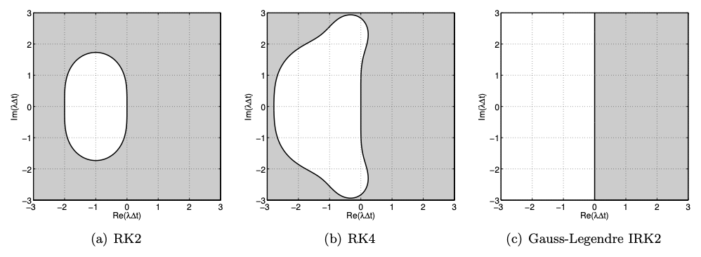
The two-stage Gauss-Legendre Runge-Kutta scheme is \(A\)-stable and is fourth-order accurate. While the method is computationally expensive and difficult to implement, the A-stability and fourth-order accuracy are attractive features for certain applications.
______________________.______________________
There is a family of implicit Runge-Kutta methods called diagonally imphicit Rtunge-Kutto (DIRK). These methods have an \(A\) matrix that is lower triangular with the same coefficients in each diagonal element. This family of methods inherits the stability advantage of IIK scheme can incrementally update the stages.
The stability diagrams for the three Runge-Kutta schemes presented are shown in Figure $21.14$. The two explicit Runge-Kutta methods, RK2 and RK4, are not $A$-stable. The time step along the real axis is limited to $-\lambda \Delta t \leq 2$ for RK2 and $-\lambda \Delta t \lesssim 2.8$ for RK4. However, the stabllity region for the explicit Runge-Kutta schemes are considerably larger than the Adams-Bashforth family of explicit schemes. While the explicit Runge-Kutta methods are not suited for very stifi systems, they can be used for moderately stiff systems. The implicit
correctly exhibits growing behavior for unstable systems.
Figure 21.15 shows the error behavior of the Runge-Kutta schemes applied to \(du/dt = −4u\). The higher accuracy of the Runge-Kutta schemes compared to the Euler Forward scheme is evident from the solution. The error convergence plot confirms the theoretical convergence rates for these methods.