21.2: Scalar Second-Order Linear ODEs

Model Problem

Let us consider a canonical second-order ODE,

\begin{aligned}
m \frac{d^{2} u}{d t^{2}}+c \frac{d u}{d t}+k u &=f(t), \quad 0<t<t_{f}, \\
u(0) &=u_{0}, \\
\frac{d u}{d t}(0) &=v_{0} .
\end{aligned}

The ODE is second order, because the highest derivative that appears in the equation is the second derivative. Because the equation is second order, we now require two initial conditions: one for displacement, and one for velocity. It is a linear ODE because the equation is linear with respect to \(u\) and its derivatives.

Figure 21.15: The error convergence behavior for the Runge-Kutta family of schemes applied to \(d^{u} u / d t=-4 u\). Here \(e(t=1)=\left|u\left(t^{j}\right)-\tilde{u}^{j}\right|\) for \(t^{j}=j \Delta t=1\).

A typical spring-mass-damper system is governed by this second-order ODE, where \(u\) is the displacement, \(m\) is the mass, \(c\) is the damping constant, \(k\) is the spring constant, and \(f\) is the external forcing. This system is of course a damped oscillator, as we now illustrate through the classical solutions.

Analytical Solution

Homogeneous Equation: Undamped

Let us consider the undamped homogeneous case, with \(c = 0\) and \(f = 0\),

\begin{aligned}
m \frac{d^{2} u}{d t^{2}}+k u &=0, \quad 0<t<t_{f}, \\
u(0) &=u_{0}, \\
\frac{d u}{d t}(0) &=v_{0} .
\end{aligned}

To solve the ODE, we assume solutions of the form \(e^{\lambda t}\), which yields

\(\left(m \lambda^{2}+k\right) e^{\lambda t}=0\).

This implies that \(m \lambda^{2}+k=0\), or that \(\lambda\) must be a root of the characteristic polynomial

\(p(\lambda)=m \lambda^{2}+k=0 \quad \Rightarrow \quad \lambda_{1,2}=\pm i \sqrt{\frac{k}{m}}\).

Let us define the natural frequency, \(\omega_{n} \equiv \sqrt{k / m}\). The roots of the characteristic polynomials are then \(\lambda_{1,2}=\pm i \omega_{n}\). The solution to the ODE is thus of the form

\(u(t)=\alpha e^{i \omega_{n} t}+\beta e^{-i \omega_{n} t}\)

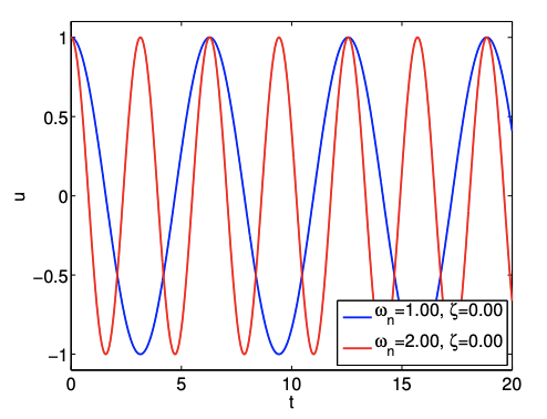
Figure 21.16: Response of undamped spring-mass systems.

Rearranging the equation,

\begin{aligned}
u(t) &=\alpha e^{i \omega_{n} t}+\beta e^{-i \omega_{n} t}=\frac{\alpha+\beta}{2}\left(e^{i \omega_{n} t}+e^{-i \omega_{n} t}\right)+\frac{\alpha-\beta}{2}\left(e^{i \omega_{n} t}-e^{-i \omega_{n} t}\right) \\
&=(\alpha+\beta) \cos \left(\omega_{n} t\right)+i(\alpha-\beta) \sin \left(\omega_{n} t\right)
\end{aligned}

Without loss of generality, let us redefine the coefficients by \(c_{1}=\alpha+\beta\) and \(c_{2}=i(\alpha-\beta)\). The general form of the solution is thus

\(u(t)=c_{1} \cos \left(\omega_{n} t\right)+c_{2} \sin \left(\omega_{n} t\right)\).

The coefficients \(c_{1}\) and \(c_{2}\) are specified by the initial condition. In particular,

\begin{aligned}
u(t=0) &=c_{1}=u_{0} & \Rightarrow & c_{1}=u_{0} \\
\frac{d u}{d t}(t=0) &=c_{2} \omega_{n}=v_{0} & \Rightarrow & c_{2}=\frac{v_{0}}{\omega_{n}}
\end{aligned}

Thus, the solution to the undamped homogeneous equation is

\(u(t)=u_{0} \cos \left(\omega_{n} t\right)+\frac{v_{0}}{\omega_{n}} \sin \left(\omega_{n} t\right)\)

which represents a (non-decaying) sinusoid.

Example 21.2.1 Undamped spring-mass system

Let us consider two spring-mass systems with the natural frequencies \(\omega_{n}=1.0\) and \(2.0\). The responses of the systems to initial displacement of \(u(t=0)=1.0\) are shown in Figure 21.16. As the systems are undamped, the amplitudes of the oscillations do not decay with time.

_______________________._______________________

Homogeneous Equation: Underdamped

Let us now consider the homogeneous case \((f = 0)\) but with finite (but weak) damping

\(m \frac{d^{2} u}{d t^{2}}+c \frac{d u}{d t}+k u=0, \quad 0<t<t_{f}\),

\begin{array}{r}
u(0)=u_{0}, \\
\frac{d u}{d t}(0)=v_{0} .
\end{array}

To solve the ODE, we again assume behavior of the form \(u=e^{\lambda e}\). Now the roots of the characteristic: polynomial are given by

\(p(\lambda)=m \lambda^{2}+c \lambda+k=0 \quad \Rightarrow \quad \lambda_{1,2}=-\frac{c}{2 m} \pm \sqrt{\left(\frac{c}{2 m}\right)^{2}-\frac{k}{m}}\).

Let us rewrite the roots as

\(\lambda_{1,2}=-\frac{c}{2 m} \pm \sqrt{\left(\frac{c}{2 m}\right)^{2}-\frac{k}{m}}=-\sqrt{\frac{k}{m}} \frac{c}{2 \sqrt{m k}} \pm \sqrt{\frac{k}{m}} \sqrt{\frac{c^{2}}{4 m k}-1}\).

For convenience, let us define the damping ratio as

\(\zeta=\frac{c}{2 \sqrt{m k}}=\frac{c}{2 m \omega_{n}}\)

Together with the definition of natural frequency, \(\omega_{n}=\sqrt{k / m}\), we can simplify the roots to

\(\lambda_{1,2}=-\zeta \omega_{n} \pm \omega_{n} \sqrt{\zeta^{2}-1}\).

The underdamped case is characterized by the condition

\(\zeta^{2}-1<0\),

i.e., \(\zeta<1\)

In this case, the roots can be conveniently expressed as

\(\lambda_{1,2}=-\zeta \omega_{n} \pm i \omega_{n} \sqrt{1-\zeta^{2}}=-\zeta \omega_{n} \pm i \omega_{d}\),

where \(\omega_{d} \equiv \omega_{n} \sqrt{1-\zeta^{2}}\) is the damped frequency. The solution to the underdamped homogeneous system is

\(u(t)=\alpha e^{-\zeta \omega_{n} t+i \omega_{d} t}+\beta e^{-\zeta \omega_{n} t-i i_{2} t} \text {. }\)

Using a similar technique as that used for the undamped case, we can simplify the expression to

\(u(t)=e^{-\zeta \Delta_{0} t}\left(c_{1} \cos \left(\omega_{d} t\right)+c_{2} \sin \left(\omega_{d} t\right)\right)\).

Substitution of the initial condition yields

\(u(t)=e^{-\zeta \omega_{n} t}\left(u_{0} \cos \left(\omega_{d} t\right)+\frac{v_{0}+\zeta \omega_{n} t_{0}}{\omega_{d}} \sin \left(\omega_{d} t\right)\right)\).

Thus, the solution is sinusoidal with exponentially decaying amplitude. The decay rate is set by the damping ratio, \(\zeta\). If \(\zeta<1\), then the oscillation decays slowly - over many periods.

Figure 21.17: Response of underdamped spring-mass-damper systems.

Example 21.2.2 Underdamped spring-mass-damper system

Let us consider two underdamped spring-mass-damper systems with

\begin{array}{ll}\text { System 1: } \quad \omega_{n}=1.0 \quad \text { and } & \zeta=0.1 \\ \text { System 2. } \quad \omega_{n}=1.0 \quad \text{ and } & \zeta=0.5 \end{array}

The responses of the systems to initial displacement of \(u(t=0)=1.0\) are shown in Figure 21.17. Unlike the undamped systems considered in Example 21.2.1, the amplitude of the cocillations decays with time; the oscillation of System 2 with a higher damping coeflictent decays quicker than that of System 1.

_______________________._______________________

Homogeneous Equation: Overdamped

In the underdamped case, we assumed \(\zeta<1\). If \(\zeta>1\), then we have an overdamped system. In this case, we write the roots as

\(\lambda_{1,2}=-\omega_{n}\left(\zeta \pm \sqrt{\zeta^{2}-1}\right)\)

both of which are real. The solution is then given by

\(u(t)=c_{1} e^{\lambda_{1} t}+c_{2} e^{\lambda_{2} t}\).

The substitution of the initial conditions yields

\(c_{1}=\frac{\lambda_{2} u_{0}-t_{0}}{\lambda_{2}-\lambda_{1}} \text { and } c_{2}=\frac{-\lambda_{1} u_{0}+v_{0}}{\lambda_{2}-\lambda_{1}}\).

The solution is a linear combination of two exponentials that decay with time constants of \(1 /\left|\lambda_{1}\right|\) and \(1 /\left|\lambda_{2}\right|\), respectively. Because \(\left|\lambda_{1}\right|>\left|\lambda_{2}\right|,\left|\lambda_{2}\right|\) dictates the long time decay behavior of the system. For \(\zeta \rightarrow \infty, \lambda_{2}\) behaves as \(-\omega_{n} /(2 \zeta)=-k / c\).

Example 21.2.3 Overdamped spring-mass-damper system

Let us consider two overdamped spring-mass-damper systems with

\begin{array}{ll}\text { System 1: } \quad \omega_{n}=1.0 \quad \text { and } & \zeta=0.1 \\ \text { System 2. } \quad \omega_{n}=1.0 \quad \text{ and } & \zeta=0.5 \end{array}

Figure 21.18: Response of overdamped spring-mass-damper systems.

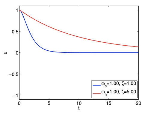
The responses of the systems to initial displacement of \(u(t = 0) = 1.0\) are shown in Figure 21.17. As the systems are overdamped, they exhibit non-oscillatory behaviors. Note that the oscillation of System 2 with a higher damping coefficient decays more slowly than that of System 1. This is in contrast to the underdamped cases considered in Example 21.2.2, in which the oscillation of the system with a higher damping coefficient decays more quickly.

_______________________._______________________

Sinusoidal Forcing

Let us consider a sinusoidal forcing of the second-order system. In particular, we consider a system of the form

\(m \frac{d^{2} u}{d t^{2}}+c \frac{d u}{d t}+k u=A \cos (\omega t)\).

In terms of the natural frequency and the damping ratio previously defined, we can rewrite the system as

\(\frac{d^{2} u}{d t^{2}}+2 \zeta \omega_{n} \frac{d u}{d t}+\omega_{n}^{2} u=\frac{A}{m} \cos (\omega t)\)

A particular solution is of the form

\(u_{p}(t)=\alpha \cos (\omega t)+\beta \sin (\omega t)\)

Substituting the assumed form of particular solution into the governing equation, we obtain

\begin{aligned}
0=& \frac{d^{2} u_{p}}{d t^{2}}+2 \zeta \omega_{n} \frac{d u_{p}}{d t}+\omega_{n}^{2} u_{p}-\frac{A}{m} \cos (\omega t) \\
=&-\omega \omega^{2} \cos (\omega t)-\beta \omega^{2} \sin (\omega t)+2 \zeta \omega_{n}(-\alpha \omega \sin (\omega t)+\beta \omega \cos (\omega t)) \\
&+\omega_{n}^{2}(\alpha \cos (\omega t)+\beta \sin (\omega t))-A \cos (\omega t)
\end{aligned}

Figure 21.19: The variation in the amplification factor for the sinusoidally forced system.

We next match terms in sin and cos to obtain

\(\alpha\left(\omega_{n}^{2}-\omega^{2}\right)+\beta\left(2 \zeta \omega \omega_{n}\right)=\frac{A}{m}\),

\(\beta\left(\omega_{n}^{2}-\omega^{2}\right)-\alpha\left(2 \zeta \omega \omega_{n}\right)=0 \text {, }\)

and solve for the coefficients,

\begin{aligned}
&\alpha=\frac{\left(\omega_{n}^{2}-\omega^{2}\right)}{\left(\omega_{n}^{2}-\omega^{2}\right)^{2}+\left(2 \zeta \omega \omega_{n}\right)^{2}} \frac{A}{m}=\frac{1-r^{2}}{\left(1-r^{2}\right)^{2}+(2 \zeta r)^{2}} \frac{A}{m \omega_{n}^{2}}=\frac{1-r^{2}}{\left(1-r^{2}\right)^{2}+(2 \zeta r)^{2}} \frac{A}{k}, \\
&\beta=\frac{\left(2 \zeta \omega \omega_{n}\right)}{\left(\omega_{n}^{2}-\omega^{2}\right)^{2}+\left(2 \zeta \omega \omega_{n}\right)^{2}} \frac{A}{m}=\frac{2 \zeta r}{\left(1-r^{2}\right)^{2}+(2 \zeta r)^{2}} \frac{A}{m \omega \omega_{n}^{2}}=\frac{2 \zeta r}{\left(1-r^{2}\right)^{2}+(2 \zeta r)^{2}} \frac{A}{k},
\end{aligned}

where \(r \equiv \omega / \omega_{n}\) is the ratio of the forced to natural frequency.

Using a trigonometric identity, we may compute the amplitude of the particular solution as

\(A_{p}=\sqrt{\alpha^{2}+\beta^{2}}=\frac{\sqrt{\left(1-r^{2}\right)^{2}+(2 \zeta r)^{2}}}{\left(1-r^{2}\right)^{2}+(2 \zeta r)^{2}} \frac{A}{k}=\frac{1}{\sqrt{\left(1-r^{2}\right)^{2}+(2 \zeta r)^{2}}} \frac{A}{k}\).

Note that the magnitude of the amplification varies with the frequency ratio, \(r\), and the damping ratio, \(\zeta\). This variation in the amplification factor is plotted in Figure 21.19. For a given \(\zeta\), the 1/(26). This increase in the magnitude of oscillation near the natural frequency of the system is known as resonance. The natural frequency is clearly crucial in understanding the forced response of the system, in particular for lightly damped systems.