21.3: System of Two First-Order Linear ODEs

It is possible to directly numerically tackle the second-order system of Section 21.2 for example much more general and in fact is the basis for numerical solution of systems of ODEs of virtually any kind.

State Space Representation of Scalar Second-Order ODEs

In this section, we develop a state space representation of the canonical second-order ODE. Recall that the ODE of interest is of the form

\(\frac{d^{2} u}{d t^{2}}+2 \zeta \omega_{n} \frac{d u}{d t}+\omega_{n}^{2} u=\frac{1}{m} f(t), \quad 0<t<t_{f}\),

\begin{aligned}
u(0) &=u_{0}, \\
\frac{d u}{d t}(0) &=v_{0} .
\end{aligned}

Because this is a second-order equation, we need two variables to fully describe the state of the system. Let us choose these state variables to be

\(w_{1}(t)=u(t) \text { and } w_{2}(t)=\frac{d u}{d t}(t)\),

corresponding to the displacement and velocity, respectively. We have the trivial relationship between \(w_1\) and \(w_2\)

\(\frac{d w_{1}}{d t}=\frac{d u}{d t}=w_{2}\).

Furthermore, the governing second-order ODE can be rewritten in terms of \(w_{1}\) and \(w_{2}\) as

\(\frac{d \omega_{2}}{d t}=\frac{d}{d t} \frac{d u}{d t}=\frac{d^{2} u}{d t^{2}}-2 \zeta \omega_{n} \frac{d u}{d t}=-\omega_{n}^{2} u+\frac{1}{m} f=-2 \zeta \omega_{n} w_{2}-\omega_{n}^{2} w_{1}+\frac{1}{m} f\).

Together, we can rewrite the original second-order ODE as a system of two first-order ODEs,

\(\dfrac{d}{d t}\left(\begin{array}{c}
w_{1} \\
w_{2}
\end{array}\right)=\left(\begin{array}{c}
w_{2} \\
-w_{n}^{2} w_{1}-2 \zeta w_{n} w_{2}+\frac{1}{m} f
\end{array}\right)\).

This equation can be written in the matrix form

\[\frac{d}{d t}\left(\begin{array}{l}
w_{1} \\
w_{2}
\end{array}\right)=\underbrace{\left(\begin{array}{cc}
0 & 1 \\
-\omega_{n}^{2} & -2 \zeta \omega_{n}
\end{array}\right)}_{A}\left(\begin{array}{c}
w_{1} \\
w_{2}
\end{array}\right)+\left(\begin{array}{c}
0 \\
\frac{1}{m} f
\end{array}\right) \tag{21.2}\]

with the initial condition

\(w_{1}(0)=u_{0} \text { and } w_{2}(0)=w_{n}\)

If we define \(w=\left(w_{1} \quad w_{2}\right)^{\mathrm{T}}\) and \(F=\left(\begin{array}{ll}0 & \frac{1}{m} f\end{array}\right)^{\mathrm{T}}\), then

\[\frac{d w}{d t}=A w+F, \quad w(t=0)=w_{0}=\left(\begin{array}{l}
u_{0} \\
v_{0}
\end{array}\right) \tag{21.3} \],

succinctly summarizes the "state-space" representation of our ODE

Solution by Modal Expansion

To solve this equation, we first find the eigenvalues of \(A\). We recall that the eigenvalues are the roots of the characteristaic equation \(p(\lambda ; A)=\) det( \((\lambda I-A)\), where det refers to the determinant. (In actual practice for large systems the eigenvalues are not computed from the characteristic equation.

In our 2 × 2 case we obtain

\(p(\lambda ; A)=\operatorname{det}(\lambda I-A)=\operatorname{det}\left(\begin{array}{cc}
\lambda & -1 \\
\omega_{n}^{2} & \lambda+2 \zeta \omega_{n}
\end{array}\right)=\lambda^{2}+2 \zeta \omega_{n} \lambda+\omega_{n}^{2} \).

The eigenvalues, the roots of characteristic equation, are thus

\(\lambda_{1,2}=-\zeta \omega_{n} \pm \omega_{n} \sqrt{\zeta^{2}-1}\).

We shall henceforth assume that the system is underdamped (i.e., \(\zeta<1\) ), in which case it is more convenient to express the eigenvalues as

\(\lambda_{1,2}=-\zeta \omega_{n} \pm i \omega_{n} \sqrt{1-\zeta^{2}} \)

Note since the eigenvalue has non-zero imaginary part the solution will be oscillatory and since the real part is negative (left-hand of the complex plane) the solution is stable. We now consider the eigenvectors.

Towards that end, we first generalize our earler discussson of vectors of real-valued components to the case of vectors of complex-valued components. To wit, if we are given two vectors \(v \in \mathbb{C}^{m \times 1}\), \(w \in \mathbb{C}^{m \times 1}-v\) and \(w\) are each column vectors with \(m\) complex entries \(-\) the inner product is now given by

\[\beta=v^{\mathrm{H}_{w}} w=\sum_{j=1}^{m} v_{j}^{*} w_{j} \tag{21.4} \],

where \(\beta\) is in general complex, \(H\) stands for Hermitian (complex transpose) and replaces T for transpose, and " denotes complex conjugate \(-80 v_{j}=\operatorname{Real}\left(v_{j}\right)+i \operatorname{Imag}\left(v_{j}\right)\) and \(v_{j}^{*}=\operatorname{Real}\left(v_{j}\right)-\)
\(i \operatorname{Imag}\left(v_{j}\right)\), for \(i=\sqrt{-1}\).

The various concepts built on the inner product change in a similar fashion. For example, two complex-valued vectors \(v\) and \(w\) are orthogonal if \(v^{\mathrm{H}} w=0\). Most importantly, the norm of complex-valued vector is now given by

\[\|v\|=\sqrt{v^{\mathbb{H}_{v}}}=\left(\sum_{j=1}^{m} v_{j}^{*} v_{j}\right)^{1 / 2}=\left(\sum_{j=1}^{m}\left|v_{j}\right|^{2}\right)^{1 / 2} \tag{21.5} \],

where \(|\cdot|\) denotes the complex modulus; \(\left|v_{j}\right|^{2}=v_{j}^{*} v_{j}=\left(\operatorname{Real}\left(v_{j}\right)\right)^{2}+\left(\operatorname{Imag}\left(v_{j}\right)\right)^{2}\). Note the definition (21.5) of the norm ensures that \(\|v\|\) is a non-negative real number, as we would expect of a length.

To obtain the eigenvectors, we must find a solution to the equation

\[(\lambda I-A) X=0 \tag{21.6} \]

for \(\lambda=\lambda_{1}\left(\Rightarrow\right.\) eigenvector \(\chi^{1} \in \mathbb{C}^{2}\) ) and \(\lambda=\lambda_{2}\) ( \(\Rightarrow\) eigenvector \(\chi^{2} \in \mathbb{C}^{2}\) ). The equations (21.6) will have a solution since \(\lambda\) has been chosen to make \((\lambda I-A)\) singular: the columns of \(\lambda I-A\) are \(x \neq 0\), of the columns of \(\lambda I-A\) which ylelds the zero vector.

Proceeding with the first eigenvector, we write \(\left(\lambda_{1} I-A\right) \chi^{1}=0\) as

\(\left(\begin{array}{cc}
-\zeta \omega_{n}+i \omega_{n} \sqrt{1-\zeta^{2}} & -1 \\
\omega_{n}^{2} & \zeta \omega_{n}+i \omega_{n} \sqrt{1-\zeta^{2}}
\end{array}\right)\left(\begin{array}{l}
\chi_{1}^{1} \\
\chi_{2}^{1}
\end{array}\right)=\left(\begin{array}{l}
0 \\
0
\end{array}\right)\)

to obtain (say, setting \(\chi_{1}^{1}=c\) ),

\(\chi^{1}=c\left(\begin{array}{c}
1 \\
\frac{-\omega_{n}^{2}}{\omega_{n}+i \omega_{n} \sqrt{1-\zeta^{2}}}
\end{array}\right) \).

We now choose \(c\) to achieve \(\left\|x^{1}\right\|=1\), yielding

\(x^{1}=\frac{1}{\sqrt{1+\omega_{n}^{2}}}\left(\begin{array}{c}
1 \\
-\zeta \omega_{n}+i \omega_{n} \sqrt{1-\zeta^{2}}
\end{array}\right)\).

In a similar fashion we obtain from \(\left(\lambda_{2} I-A\right) \chi^{2}=0\) the second eigenvector

\(x^{2}=\frac{1}{\sqrt{1+\omega_{n}^{2}}}\left(\begin{array}{c}
1 \\
-\zeta \omega_{n}-i \omega_{n} \sqrt{1-\zeta^{2}}
\end{array}\right)\)

which satisfies \(\left\|x^{2}\right\|=1\).

We now introduce two additional vectors, \(\psi^{1}\) and \(\psi^{2}\). The vector \(\psi^{1}\) is chosen to satisfy \(\left(\psi^{1}\right)^{\mathrm{H}} \chi^{2}=0\) and \(\left(\psi^{1}\right)^{\mathrm{H}} \chi^{1}=1\), while the vector \(\psi^{2}\) is chosen to satisfy \(\left(\psi^{2}\right)^{\mathrm{H}^{\mathrm{H}}} \chi^{1}=0\) and \(\left(\psi^{2}\right)^{\mathrm{H}} \chi^{2}=\)1. We find, after a little algebra,

\(\psi^{1}=\frac{\sqrt{1+\omega_{n}^{2}}}{2 i \omega_{n} \sqrt{1-\zeta^{2}}}\left(\begin{array}{c}
-\zeta \omega_{n}+i \omega_{n} \sqrt{1-\zeta^{2}} \\
-1
\end{array}\right), \psi^{2}=\frac{\sqrt{1+\omega_{n}^{2}}}{-2 i \omega_{n} \sqrt{1-\zeta^{2}}}\left(\begin{array}{c}
-\zeta \omega_{n}-i \omega_{n} \sqrt{1-\zeta^{2}} \\
-1
\end{array}\right) \).

These choices may appear mysterious, but in a moment we will see the utility of this “bi-orthogonal” system of vectors. (The steps here in fact correspond to the “diagonalization” of \(A\).)

We now write \(w\) as a linear combination of the two eigenvectors, or “modes,”

\[\begin{array}{rl}w(t) & =z_{1}(t) \chi^{1}+z_{2}(t) \chi^{2} \\ & =S z(t) \end{array} \tag{21.7}\]

where

\(S = \left(\chi^{1} \chi^{2}\right)\)

is the \(2 \times 2\) matrix whose \(j^{\text {th }}\)-column is given by the \(j^{\text {th-eigenvector, } \chi^{j}}\). We next insert (21.7) into (21.3) to obtain

\[\chi^{1} \frac{d z_{1}}{d t}+\chi^{2} \frac{d z_{2}}{d t}=A\left(\chi^{1} z_{1}+\chi^{2} z_{2}\right)+F \tag{21.8}\]

\[\left(\chi^{1} z_{1}+\chi^{2} z_{2}\right)(t=0)=w_{0} \tag{21.9}\]

We now take advantage of the \(\psi\) vectors.

First we multiply (21.8) by \(\left(\psi^{1}\right)^{\mathrm{H}}\) and take advantage of \(\left(\psi^{1}\right)^{\mathrm{H}} \chi^{2}=0,\left(\psi^{1}\right)^{\mathrm{H}} \chi^{1}=1\), and \(A \chi^{j}=\lambda_{j} \chi^{j}\) to obtain

\[\frac{d z_{1}}{d t}=\lambda_{1} z_{1}+\left(\psi^{1}\right)^{\mathrm{H}} F \tag{21.10}\]

if we similarly multiply (21.9) we obtain

\[z_1 \left( t=0 \right) = \left( \psi \right)^{\mathrm{H}}w_0 \tag{21.11}\]

The same procedure but now with \(\left(\psi^{2}\right)^{\mathrm{H}}\) rather than \(\left(\psi^{1}\right)^{\mathrm{H}}\) gives

\[\frac{d z_{2}}{d t}=\lambda_{2} z_{2}+\left(\psi^{2}\right)^{\mathrm{H}} F \tag{21.12}\];

\[z_{2}(t=0)=\left(\psi^{2}\right)^{\mathrm{H}} w_{0} \tag{21.13}\]

We thus observe that our modal expansion reduces our coupled \(2 \times 2\) ODE system into two decoupled ODEs.

The fact that \(\lambda_{1}\) and \(\lambda_{2}\) are complex means that \(z_{1}\) and \(z_{2}\) are also complex, which might appear inconsistent with our original real equation (21.3) and real solution \(w(t)\). However, we note that \(\lambda_{2}=\lambda_{1}^{*}\) and \(\psi^{2}=\left(\psi^{1}\right)^{*}\) and thus \(z_{2}=z_{1}^{*}\). It thus follows from (21.7) that, since \(\chi^{2}=\left(\chi^{1}\right)^{*}\) as well,

\(w=z_{1} \chi^{1}+z_{1}^{*}\left(\chi^{1}\right)^{*}\)

and thus

\(w=2 \operatorname{Real}\left(z_{1} x^{1}\right)\).

Upon superposition, our solution is indeed real, as desired. interest here in the modal decomposition is as a way to understand how to choose an ODE scheme for a system of two (later \(n\) ) ODEs, and, for the chosen scheme, how to choose \(\Delta t\) for stability.

Numerical Approximation of a System of Two ODEs

Crank-Nicolson

The application of the Crank-Nicolson scheme to our system (21.3) is identical to the application of the Crank-Nicolson scheme to a scalar ODE. In particular, we directly take the scheme of example 21.1.8 and replace \(\tilde{u}^j \in \mathbb{R}\) with \(\tilde{w}^j \in \mathbb{R}^2\) and \(g\) with \(A \tilde{w}^j + F^j\) to obtain

\[\tilde{w}^{j}=\tilde{w}^{j-1}+\frac{\Delta t}{2}\left(A \tilde{w}^{j}+A \tilde{w}^{j-1}\right)+\frac{\Delta t}{2}\left(F^{j}+F^{j-1}\right) \tag{21.14}\].

(Note if our force \(f\) is constant in time then \(F^{j}=F\).) In general if follows from consistency arguments that we will obtain the same order of convergence as for the scalar problem - if (21.14) is stable. The diffeult issue for systems is stability: Will a particular scheme have good stability scheme be stable? (The latter is particularly important for explicit schemes.)

To address these questions we again apply modal analysis but now to our discrete equations (21.14). In particular, we write

\[\tilde{w}^{j}=\tilde{z}_{1}^{j} x^{1}+\bar{z}_{2}^{j} x^{2} \tag{21.15}\],

where \(\chi^{1}\) and \(x^{2}\) are the eigenvectors of \(A\) as derived in the previous section. We now insert (21.15) into (21.14) and multiply by \(\left(\psi^{1}\right)^{\mathrm{H}}\) and \(\left(\psi^{2}\right)^{\mathrm{H}}-\) just as in the previous section \(-\) to obtain

\[z_{1}^{j}=z_{1}^{j-1}+\frac{\lambda_{1} \Delta t}{2}\left(\tilde{z}_{1}^{j}+z_{1}^{j-1}\right)+\left(\psi^{1}\right)^{\mathrm{H}} \frac{\Delta t}{2}\left(F^{j}+F^{j-1}\right) \tag{21.16}\],

\[z_{2}^{j}=z_{2}^{j-1}+\frac{\lambda_{2} \Delta t}{2}\left(z_{2}^{j}+z_{2}^{j-1}\right)+\left(\psi^{2}\right)^{\mathrm{H}} \frac{\Delta t}{2}\left(F^{j}+F^{j-1}\right) \tag{21.17}\],

with corresponding initial conditions (which are not relevant to our current discussion).

We now recall that for the model problem

\[\dfrac{d u}{d t}=\lambda u+f \tag{21.18}\],

analogous to (21.10), we arrive at the Crank-Nicolson scheme

\[\tilde{u}^{j}=\tilde{u}^{j-1}+\frac{\lambda \Delta t}{2}\left(\tilde{u}^{j}+\tilde{w}^{j-1}\right)+\frac{\Delta t}{2}\left(f^{j}+f^{j-1}\right) \tag{21.19}\],

analogous to (21.16). Working backwards, for (21.19) and hence (21.16) to be a stable approximation to (21.18) and hence (21.10), we must require \(\lambda \Delta t\), and hence \(\lambda_{1} \Delta t\), to reside in the that the difference equation (21.16) will blow up - and hence also (21.14) by virture of (21.15) - if \(\lambda_{1} \Delta t\) is not in the unshaded region of Figure 21.12(a). By similar arguments, \(\lambda_{2} \Delta t\) must also lie in the unshaded region of Figure 21.12(a). In this case, we know that both \(\lambda_{1}\) and \(\lambda_{2}\)-for our particular equation, that is, for our particular matrix \(A\) (which determines the eigenvalues \(\lambda_{1}\), \(\left.\lambda_{2}\right)\) - are in the left-hand plane, and hence in the Crank-Nicolson absolute stability region; thus Crank-Nicolson is unconditionally stable — stable for all \(\Delta t\) - for our particular equation and will converge as \(O\left(\Delta t^{2}\right)\) as \(\Delta t \rightarrow 0\).

We emphasize that the numerical procedure is given by (21.14), and not by (21.16), (21.17). The modal decompositjon is just for the purposes of understanding and analysis - to determine if a scheme is stable and if so for what values of \(\Delta t\). (For a \(2 \times 2\) matrix \(A\) the full modal decomposition is simple. But for larger systems, as we will consider in the next section, the full modal decomposition is very expensive. Hence we prefer to directly discretize the original equation, as in (21.14). This that \(\Delta t\) in (21.16) and (21.17) are the same - both originate in the equation (21.14). We discuss this further below in the context of stiff equations.

General Recipe

We now consider a general system of \(n=2\) ODEs given by

\[\frac{d w}{d t}=A w+F \tag{21.20}\],

\[w(0)=w_{0} \tag{21.20}\]

where \(w \in \mathbb{R}^{2}, A \in \mathbb{R}^{2 \times 2}\) (a \(2 \times 2\) matrix), \(F \in \mathbb{R}^{2}\), and \(w 0 \in \mathbb{R}^{2}\). We next discretize (21.20) by any of the schemes developed earlier for the scalar equation

\(\dfrac{d u}{d t}=g(u, t)\)

simply by substituting \(w\) for \(u\) and \(Aw + F\) for \(g(u, t)\). We shall denote the scheme by \(\mathbb{S}\) and the associated absolute stability region by \(\mathcal{R}_{\mathbb{S}}\). Recall that (\mathcal{R}_{\mathbb{S}}\) is the subset of the complex plane which contains all \(\lambda \Delta t\) for which the scheme \(\mathbb{S}\) applied to \(g(u, t) = \lambda u\) is absolutely stable.

For example, if we apply the Euler Forward scheme \(\mathbb{S}\) we obtain

\[\tilde{w}^{j}=\tilde{w}^{j-1}+\Delta t\left(A \tilde{w}^{j-1}+F^{j-1}\right) \tag{21.21}\]

whereas Euler Backward as \(\mathbb{S}\) yields

\[\tilde{w}^{j}=\tilde{w}^{j-1}+\Delta t\left(A \tilde{w}^{j}+F^{j}\right) \tag{21.22}\],

and Crank-Nicolson as \(\mathbb{S}\) gives

\[\tilde{w}^{j}=\tilde{w}^{j-1}+\frac{\Delta t}{2}\left(A \tilde{w}^{j}+A \tilde{w}^{j-1}\right)+\frac{\Delta t}{2}\left(F^{j}+F^{j-1}\right) \tag{21.23}\] .

A multistep scheme such as AB2 as \(\mathbb{S}\) gives

\[\tilde{w}^{j}=\tilde{w}^{j-1}+\Delta t\left(\frac{3}{2} A \tilde{w}^{j-1}-\frac{1}{2} A \tilde{w}^{j-2}\right)+\Delta t\left(\frac{3}{2} F^{j-1}-\frac{1}{2} F^{j-2}\right) \tag{21.24}\]

The stability diagrams for these four schemes, \(\mathcal{R}_{\mathbb{S}}\), are given by Figure 21.9, Figure 21.7, Figure 21.12(a), and Figure 21.11(b), respectively.

We next assume that we can calculate the two eigenvalues of \(A, \lambda_{1}\), and \(\lambda_{2}\). A particular \(\Delta t\) will lead to a stable scheme if and only if the two points \(\lambda_{1} \Delta t\) and \(\lambda_{2} \Delta t\) both lie inside \(\mathcal{R}_{\mathbb{S}}\). If either or both of the two points \(\lambda_{1} \Delta t\) or \(\lambda_{2} \Delta t\) lie outside \(\mathcal{R}_{\mathbb{S}}\), then we must decrease \(\Delta t\) until both \(\lambda_{1} \Delta t\) and \(\lambda_{2} \Delta t\) lie inside \(\mathcal{R}_{\mathbb{S}}\). The critical time step, \(\Delta t_{\mathrm{cr}}\), is defined to be the largest \(\Delta t\) for which the two rays \(\left[0, \lambda_{1} \Delta t\right],\left[0, \lambda_{2} \Delta t\right]\), both lie within \(\mathcal{R}_{\mathbb{S}} ; \Delta t_{\mathrm{cr}}\) will depend on the shape and size of \(\mathcal{R}_{\mathbb{S}}\) and the "orientation" of the two rays \(\left[0, \lambda_{1} \Delta t\right],\left[0, \lambda_{2} \Delta t\right]\).

We can derive \(\Delta t_{\mathrm{cr}}\) in a slightly different fashion. We first define \(\widehat{\Delta t}_{1}\) to be the largest \(\Delta t\) such that the ray \(\left[0, \lambda_{1} \Delta t\right]\) is in \(\mathcal{R}_{\mathbb{S}}\); we next define \(\widehat{\Delta t}_{2}\) to be the largest \(\Delta t\) such that the ray \(\left[0, \lambda_{2} \Delta t\right]\) is in \(\mathcal{R}_{\mathbb{S}}\). We can then deduce that \(\Delta t_{\mathrm{cr}}=\min \left(\widehat{\Delta t}_{1}, \widehat{\Delta t}_{2}\right)\). In particular, we note that if \(\Delta t>\Delta t_{\mathrm{cr}}\) then one of the two modes - and hence the entire solution - will explode. We can also see here again the difficulty with stiff equations in which \(\lambda_{1}\) and \(\lambda_{2}\) are very different: \(\widehat{\Delta t} t_{1}\) may be (say) much larger than \(\widehat{\Delta t}_{2}\), but \(\widehat{\Delta t}_{2}\) will dictate \(\Delta t\) and thus force us to take many time steps - many more than required to resolve the slower mode (smaller \(\left|\lambda_{1}\right|\) associated with slower decay or slower oscillation) which is often the behavior of interest.

In the above we assumed, as is almost always the case, that the \(\lambda\) are in the left-hand plane. For any $\lambda$ which are in the right-hand plane, our condition is flipped: we now must make sure that the \(\lambda \Delta t\) are not in the absolute stability region in order to obtain the desired growing (unstable) solutions.

Let us close this section with two examples.

Example 21.3.1 Undamped spring-mass system

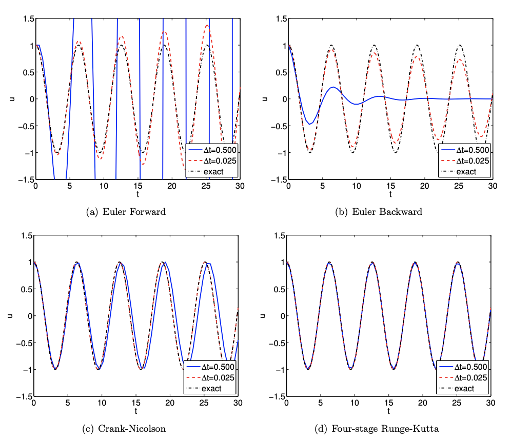
In this example, we revisit the undamped spring-mass system considered in the previous section. The two eigenvalues of \(A\) are \(\lambda_{1}=i \omega_{n}\) and \(\lambda_{2}=i \omega_{n}\); without loss of generality, we set \(\omega_{n}=1.0\). We will consider application of several different numerical integration schemes to the problem; for each integrator, we assess its applicability based on theory (by appealing to the absolute stability diagram) and verify our assessment through numerical experiments.

\((i)\) Euler Forward is a poor choice since both \(\lambda_{1} \Delta t\) and \(\lambda_{2} \Delta t\) are outside \(\mathcal{R}_{\mathbb{S}=E F}\) for all \(\Delta t\). The result of numerical experiment, shown in Figure 21.20(a), confirms that the amplitude of the oscillation grows for both \(\Delta t=0.5\) and \(\Delta t=0.025\); the smaller time step results in a smaller (artificial) amplification.

\((ii)\) Euler Backward is also a poor choice since $\lambda_{1} \Delta t$ and $\lambda_{2} \Delta t$ are in the interior of $\mathcal{R}_{\mathrm{S}=\text { EB }}$ for all $\Delta t$ and hence the discrete solution will decay even though the exact solution is a non-decaying oscillation. Figure 21.20(b) confirms the assessment.

\((iii)\) Crank-Nicolson is a very good choice since \(\lambda_{1} \Delta t \in \mathcal{R}_{\mathrm{S}=\mathrm{CN}}, \lambda_{2} \Delta t \in \mathcal{R}_{\mathrm{S}=\mathrm{CN}}\) for all \(\Delta t\), and furthermore \(\lambda_{1} \Delta t, \lambda_{2} \Delta t\) lie on the boundary of \(\mathcal{R}_{S=\mathrm{CN}}\) and hence the discrete solution, just as the exact solution, will not decay. Figure 21.20(c) confirms that Crank-Nicolson preserves results in a noticeable phase error.

\((iv)\) Four-stage Runge-Kutta (RK4) is a reasonably good choice since \(\lambda_{1} \Delta t\) and \(\lambda_{2} \Delta t\) lie close to the boundary of \(\mathcal{R}_{\mathbb{S} = \rm RK4}\) for \(| \lambda_i \Delta t | \lesssim 1\). Figure 21.20(d) shows that, for the problem considered, RK4 excels at not only preserving the amplitude of the oscillation but also at attaining the correct phase.

Note in the above analysis the absolute stability diagram serves not only to determine stability but also the nature of the discrete solution as regards growth, or decay, or even neutral stability - no growth or decay. (The latter does not imply that the discrete solution is exact, since in addition to in particular demonstrate the presence of phase errors in the absence of amplitude errors.)

Figure 21.20: Comparison of numerical integration schemes for an undamped spring-mass system with \(ω_n = 1.0\).

Example 21.3.2 Overdamped spring-mass-damper system: a stiff system of ODEs

In our second example, we consider a (very) overdamped spring-mass-damper system with \(\omega_{n}=1.0\) and \(\zeta=100\). The eigenvalues associated with the system are

\begin{aligned}
&\lambda_{1}=-\zeta \omega_{n}+\omega_{n} \sqrt{\zeta^{2}-1}=-0.01 \\
&\lambda_{2}=-\zeta \omega_{n}-\omega_{n} \sqrt{\zeta^{2}-1}=-99.99 .
\end{aligned}

As before, we perturb the system by a unit initial displacement. The slow mode with $\lambda_{1}=-0.01$ dictates the response of the system. However, for conditionally stable schemes, the stability is governed by the fast mode with \(\lambda_2 = −99.99\). We again consider four different time integrators: two explicit and two implicit.

\((i)\) Euler Forward is stable for \(\Delta t \lesssim 0.02\) (i.e. \(\Delta t_{\mathrm{cc}}=2 /\left|\lambda_{2}\right|\) ). Figure 21.21(a) shows that the scheme accurately tracks the (rather benign) exact solution for \(\Delta t=0.02\), but becomes unstable and diverges exponentially for \(\Delta t=0.0201\). Thus, the maximum time step is limited (dictated by \(\lambda_{2}\) ). In other words, even though the system response is benign, we cannot use large tíme steps to save on computational cost.

\((ii)\) Similar to the Euler Forward case, the four-stage Runge-Kutta (RK4) scheme exhibits an exponentially diverging behavior for \(\Delta t>\Delta t_{\mathrm{cr}} \approx 0.028\), as shown in Figure 21.21(b). The maximum time step is again limited by stability.

\((iii)\) Euler Backward is unconditionally stable, and thus the choice of the time step is dictated by the ability to approximate the system response, which is dictated by \(\lambda_{1}\). Figure 21.21(c) large as \(\Delta t=5.0\) since the system response is rather slow.

\((iv)\) Crank-Nicolson is also unconditionally stable. For the same set of time steps, Crank-Nicolson produces a more accurate approximation than Euler Backward, as shown in Figure 21.21(d), due to its higher-order accuracy.

In the above comparison, the unconditionally stable schemes required many fewer time steps (and bence much less computational effort) than conditionally stable schemes. For instance, Crank Nicolson with \(\Delta t=5.0\) requires approximately 200 times fewer time steps than the RK4 scheme (with a stable choice of the time step). More importantly, as the shortest time scale (i.e. the largest eigenvalue) dictates stability, conditionally stable schemes do not allow the user to use large time steps even if the fast modes are of no interest to the user. As mentioned previously, stiff system are ubiquitous in engineering, and engineers are often not interested in the smallest time scale present are in the system. (Recall the example of the time scale associated with the dynamics of a passenger jet and that associated with turbulent eddies; engineers are often only interested in characterizing the dynamics of the aircraft, not the eddies.) In these situations, unconditionally stable schemes allow users to choose an appropriate time step independent of stability limitations.

___________________________.___________________________

In closing, it is clear even from these simple examples that a general purpose explicit scheme would ideally include some part of both the negative real axis and the imaginary axis. Schemes that exhibit this behavior include AB3 and RK4. Of these two schemes, RK4 is often preferred due to a large stability region; also RK4, a multi-stage method, does not suffer from the start-up issues that sometimes complicate multi-step techniques.