21.4: IVPs - System of n Linear ODEs

We consider here for simplicity a particular family of problems: \(n/2\) coupled oscillators. This family of systems can be described by the set of equations.

\begin{gathered}
\frac{d^{2} u^{(1)}}{d t^{2}}=h^{(1)}\left(\frac{d u^{(j)}}{d t}, u^{(j)}, 1 \leq j \leq n / 2\right)+f^{(1)}(t) \\
\frac{d^{2} u^{(2)}}{d t^{2}}=h^{(2)}\left(\frac{d u^{(j)}}{d t}, u^{(j)}, 1 \leq j \leq n / 2\right)+f^{(2)}(t) \\
\vdots \\
\frac{d^{2} u^{(n / 2)}}{d t^{2}}=h^{(n / 2)}\left(\frac{d u^{(j)}}{d t}, u^{(3)}, 1 \leq j \leq n / 2\right)+f^{(n / 2)}(t)
\end{gathered}

where \(h^{(k)}\) is assumed to be a linear function of all its arguments.

Figure 21.21: Comparison of numerical integration schemes for an overdamped spring-mass-damper system with \(ω_n = 1.0\) and \(ζ = 50\). Note that the time step used for the explicit schemes are different from those for the implicit schemes.

We first convert this system of equations to state space form. We identify

\(w_{1}=u^{(1)}, \quad w_{2}=\frac{d u^{(1)}}{d t}\)

\(w_{3}=u^{(2)}, \quad w_{4}=\frac{d u^{(2)}}{d t}\)

\(w_{n-1}=u^{(n / 2)}, \quad w_{n}=\frac{d u^{(n / 2)}}{d t}\)

We can then write our system - using the fact that \(h\) is linear in its arguments - as

\[\dfrac{d w}{d t}=A w+F \tag{21.25}\]

\[w(0)=w_{0} \tag{21.25}\]

where \(h\) determines \(A, F\) is given by \(\left(\begin{array}{llll}0 & f^{(1)}(t) & 0 & f^{(2)}(t) \cdots 0 f^{(n/2)}(t) \end{array}\right)^T.\)

\(w_{0}=\left(u^{(1)}(0) \frac{d u^{(1)}}{d t}(0) \quad u^{(2)}(0) \frac{d u^{(2)}}{d t}(0) \quad \ldots \quad u^{(n / 2)}(0) \frac{d u^{(n / 2)}}{d t}(0)\right)^{\mathrm{T}}\)

We have now reduced our problem to an abstract form identical to (21.20) and hence we may apply any scheme \(\mathbb{S}\) to (21.25) in the same fashion as to (21.20).

For example, Euler Forward, Euler Backward, Crank-Nicolson, and AB2 applied to (21.25) will take the same form (21.21),(21.22),(21.23),(21.24), respectively, except that now \(w \in \mathbb{R}^{n}\), \(A \in \mathbb{R}^{n \times n}, F \in \mathbb{R}^{n}, w_{0} \in \mathbb{R}^{n}\) are given in (21.25), where \(n / 2\), the number of oscillators (or masses) in our system, is no longer restricted to \(n / 2=1\) (i.e., \(n=2\) ). We can similarly apply AB3 or BD2 or RK4.

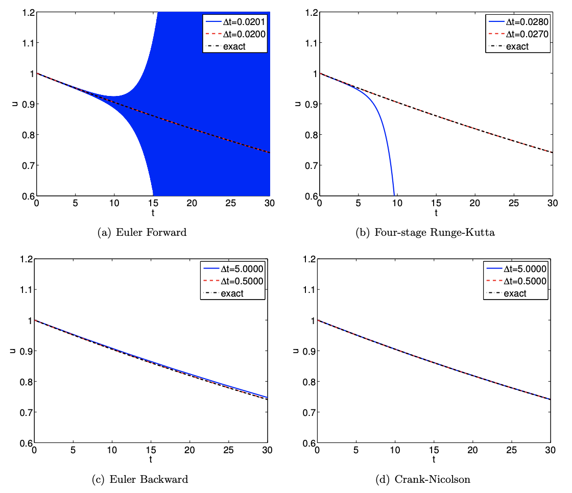
Our stability criterion is also readily extended. We first note that \(A\) will now have in general \(n\) eigenvalues, \(\lambda_{1}, \lambda_{2}, \ldots, \lambda_{n}\). (In certain cases multiple eigenvalues can create difficulties; we do not consider these typically rather rare cases here.) Our stability condition is then simply stated: a time step \(\Delta t\) will lead to stable behavior if and only if \(\lambda_{i} \Delta t\) is in \(\mathcal{R}_{\mathbb{S}}\) for all \(i, 1 \leq i \leq n\). If this condition is not satisfied then there will be one (or more) modes which will explode, taking with it (or them) the entire solution. (For certain very special initial conditions - in which the \(w_{0}\) is chosen such that all of the dangerous modes are initially exactly zero - this blow-up could be avoided in infinite precision; but in finite precision we would still be doomed.) For explicit schemes, \(\Delta t_{\mathrm{cr}}\) is the largest time step such that all the rays \(\left[0, \lambda_{i} \Delta t\right], 1 \leq i \leq n\), lie within \(\mathcal{R}_{\mathbb{S}}\).

There are certainly computational difficulties that arise for large \(n\) that are not an issue for \(n=2\) (or small \(n\) ). First, for implicit schemes, the necessary division - solution rather than evaluation of matrix-vector equations - will become considerably more expensive. Second, for explicit schemes, determination of \(\Delta t_{\mathrm{cr}}\), or a bound \(\Delta t_{\mathrm{cr}}^{\text {conservative }}\) such that \(\Delta t_{\mathrm{cr}}^{\text {conservative }} \approx t_{\mathrm{cr}}\) and \(\Delta t_{\mathrm{cr}}^{\text {conservative }} \leq \Delta t_{\mathrm{cr}}\), can be difficult. As already mentioned, the full modal decomposition can be expensive. Fortunately, in order to determine \(\Delta t_{\mathrm{cr}}\), we often only need as estimate for say the most negative real eigenvalue, or the largest (in magnitude) imaginary eigenvalue; these extreme eigenvalues can often be estimated relatively efficiently.

Finally, we note that in practice often adaptive schemes are used in which stability and accuracy are monitored and \(∆t\) modified appropriately. These methods can also address nonlinear problems — in which \(h\) no longer depends linearly on its arguments.