26.1: A 2 × 2 System (n = 2)

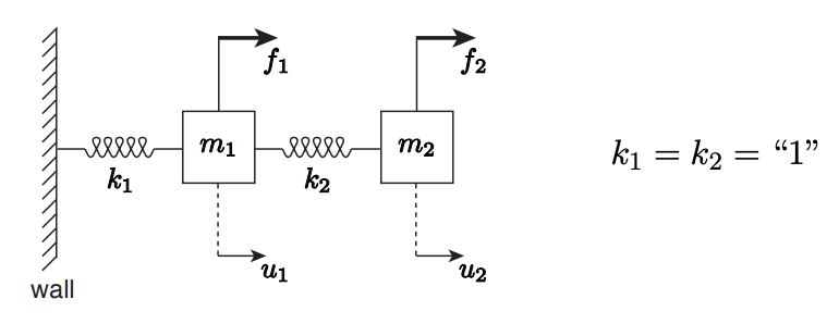
Let us revisit the two-mass mass-spring system \((n=2)\) considered in the previous chapter; the system is reproduced in Figure \(26.1\) for convenience. For simplicity, we set both spring constants to unity, i.e. \(k_{1}=k_{2}=1\). Then, the equilibrium displacement of mass \(m_{1}\) and \(m_{2}, u_{1}\) and \(u_{2}\), is described by a linear system \[\underset{(K)}{A} u=f \quad \rightarrow\left(\begin{array}{rr} 2 & -1 \\ -1 & 1 \end{array}\right)\left(\begin{array}{l} u_{1} \\ u_{2} \end{array}\right)=\left(\begin{array}{l} f_{1} \\ f_{2} \end{array}\right),\] where \(f_{1}\) and \(f_{2}\) are the forces applied to \(m_{1}\) and \(m_{2}\). We will use this \(2 \times 2\) system to describe a systematic two-step procedure for solving a linear system: a linear solution strategy based on Gaussian elimination and back substitution. While the description of the solution strategy may appear overly detailed, we focus on presenting a systematic approach such that the approach generalizes to \(n \times n\) systems and can be carried out by a computer.

Figure 26.1: \(n=2\) spring-mass system.

We recognize that we can eliminate \(u_{1}\) from the second equation by adding \(1 / 2\) of the first equation to the second equation. The scaling factor required to eliminate the first coefficient from the second equation is simply deduced by diving the first coefficient of the second equation \((-1)\) by the "pivot" - the leading coefficient of the first equation (2) - and negating the sign; this systematic procedure yields \((-(-1) / 2)=1 / 2\) in this case. Addition of \(1 / 2\) of the first equation to the second equation yields a new second equation \[\begin{aligned} u_{1}-\frac{1}{2} u_{2} &=\frac{1}{2} f_{1} \\ -u_{1}+u_{2} &=f_{2} \\ 0 u_{1}+\frac{1}{2} u_{2} &=\frac{1}{2} f_{1}+f_{2} \end{aligned} .\] Note that the solution to the linear system is unaffected by this addition procedure as we are simply adding "0" - expressed in a rather complex form - to the second equation. (More precisely, we are adding the same value to both sides of the equation.)

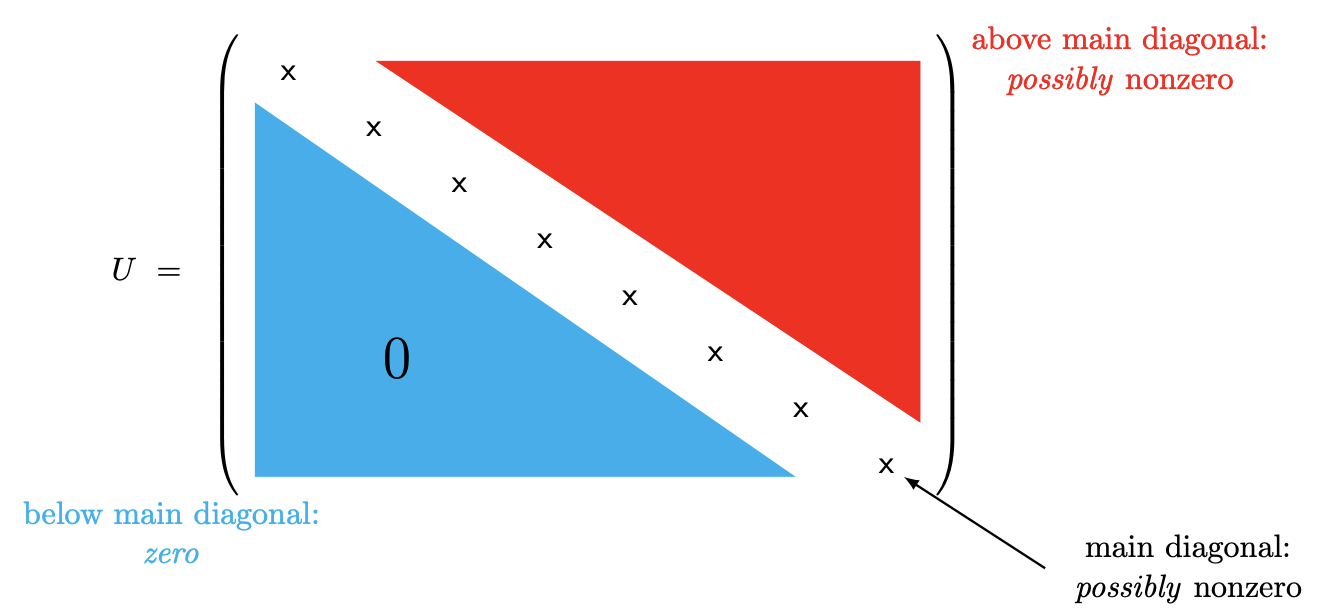
Collecting the new second equation with the original first equation, we can rewrite our system of linear equations as \[\begin{aligned} 2 u_{1}-u_{2} &=f_{1} \\ 0 u_{1}+\frac{1}{2} u_{2} &=f_{2}+\frac{1}{2} f_{1} \end{aligned}\] or, in the matrix form, \[\underbrace{\left(\begin{array}{rr} 2 & -1 \\ 0 & \frac{1}{2} \end{array}\right)}_{U} \underbrace{\left(\begin{array}{l} u_{1} \\ u_{2} \end{array}\right)}_{u}=\underbrace{\left(\begin{array}{c} f_{1} \\ f_{2}+\frac{1}{2} f_{1} \end{array}\right)}_{\hat{f}} .\] Here, we have identified the new matrix, which is upper triangular, by \(U\) and the modified righthand side by \(\hat{f}\). In general, an upper triangular matrix has all zeros below the main diagonal, as shown in Figure 26.2; the zero entries of the matrix are shaded in blue and (possibly) nonzero entries are shaded in red. For the \(2 \times 2\) case, upper triangular simply means that the \((2,1)\) entry is zero. Using the newly introduced matrix \(U\) and vector \(\hat{f}\), we can concisely write our \(2 \times 2\) linear system as \[U u=\hat{f}\] The key difference between the original system Eq. (26.1) and the new system Eq. (26.2) is that the new system is upper triangular; this leads to great simplification in the solution procedure as we now demonstrate.

First, note that we can find \(u_{2}\) from the second equation in a straightforward manner, as the equation only contains one unknown. A simple manipulation yields \[\begin{array}{ll} \text { eqn } 2 \\ \text { of } U \end{array} \quad \frac{1}{2} u_{2}=f_{2}+\frac{1}{2} f_{1} \Rightarrow u_{2}=f_{1}+2 f_{2}\] Having obtained the value of \(u_{2}\), we can now treat the variable as a "known" (rather than "unknown") from hereon. In particular, the first equation now contains only one "unknown", \(u_{1}\); again,

Figure 26.2: Illustration of an upper triangular matrix.

it is trivial to solve for the single unknown of a single equation, i.e.

\[\begin{aligned} & \begin{array}{ll}\text { eqn } 1 \\\text { of } U\end{array} \quad 2 u_{1}-u_{2}=f_{1} \\ & \Rightarrow 2 u_{1} \quad=f_{1}+\underset{\text { (already know) }}{u_{2}} \\ & \Rightarrow \quad 2 u_{1} \quad=f_{1}+f_{1}+2 f_{2}=2\left(f_{1}+f_{2}\right) \\ & \Rightarrow u_{1} \quad=\left(f_{1}+f_{2}\right) . \end{aligned}\]

Note that, even though the \(2 \times 2\) linear system Eq. (26.2) is still a fully coupled system, the solution procedure for the upper triangular system is greatly simplified because we can sequentially solve (two) single-variable-single-unknown equations.

In above, we have solved a simple \(2 \times 2\) system using a systematic two-step approach. In the first step, we reduced the original linear system into an upper triangular system; this step is called Gaussian elimination (GE). In the second step, we solved the upper triangular system sequentially starting from the equation described by the last row; this step is called back substitution (BS). Schematically, our linear system solution strategy is summarized by \[\left\{\begin{array}{lll} \text { GE: } & A u=f \Rightarrow U u=\hat{f} & \text { STEP } 1 \\ \text { BS: } & U u=\hat{f} \Rightarrow u & \text { STEP } 2 . \end{array}\right.\] This systematic approach to solving a linear system in fact generalize to general \(n \times n\) systems, as we will see shortly. Before presenting the general procedure, let us provide another concrete example using a \(3 \times 3\) system.