26.2: A 3 × 3 System (n = 3)

Figure \(26.3\) shows a three-mass spring-mass system \((n=3)\). Again assuming unity-stiffness springs

Figure 26.3: A \(n=3\) spring-mass system.

for simplicity, we obtain a linear system describing the equilibrium displacement: \[\underset{(K)}{A} u=f \rightarrow\left(\begin{array}{rrr} 2 & -1 & 0 \\ -1 & 2 & -1 \\ 0 & -1 & 1 \end{array}\right)\left(\begin{array}{l} u_{1} \\ u_{2} \\ u_{3} \end{array}\right)=\left(\begin{array}{l} f_{1} \\ f_{2} \\ f_{3} \end{array}\right) .\] As described in the previous chapter, the linear system admits a unique solution for a given \(f\).

Let us now carry out Gaussian elimination to transform the system into an upper triangular system. As before, in the first step, we identify the first entry of the first row ( 2 in this case) as the "pivot"; we will refer to this equation containing the pivot for the current elimination step as the "pivot equation." We then add \((-(-1 / 2))\) of the "pivot equation" to the second equation, i.e.

\(\begin{array}{rrrrr}2 & -1 & 0 & f_{1} & \frac{1}{2} \text { eqn 1 } \\ -1 & 2 & -1 & f_{2} & +1 \text { eqn 2 } \\ 0 & -1 & 1 & f_{3} & \end{array}\)

where the system before the reduction is shown on the left, and the operation to be applied is shown on the right. The operation eliminates the first coefficient (i.e. the first-column entry, or simply "column 1 ") of eqn 2 , and reduces eqn 2 to \[0 u_{1}+\frac{3}{2} u_{2}-u_{3}=f_{2}+\frac{1}{2} f_{1} .\] Since column 1 of eqn 3 is already zero, we need not add the pivot equation to eqn 3 . (Systematically, we may interpret this as adding \((-(0 / 2))\) of the pivot equation to eqn 3.) At this point, we have completed the elimination of the column 1 of eqn 2 through eqn \(3(=n)\) by adding to each appropriately scaled pivot equations. We will refer to this partially reduced system, as " \(U\)-to-be"; in particular, we will denote the system that has been reduced up to (and including) the \(k\)-th pivot by \(\tilde{U}(k)\). Because we have so far processed the first pivot, we have \(\tilde{U}(k=1)\), i.e. \[\tilde{U}(k=1)=\left(\begin{array}{rrr} 2 & -1 & 0 \\ 0 & \frac{3}{2} & -1 \\ 0 & -1 & 1 \end{array}\right)\] In the second elimination step, we identify the modified second equation (eqn \(2^{\prime}\) ) as the "pivot equation" and proceed with the elimination of column 2 of eqn \(3^{\prime}\) through eqn \(n^{\prime}\). (In this case, we modify only eqn \(3^{\prime}\) since there are only three equations.) Here the prime refers to the equations in \(\tilde{U}(k=1)\). Using column 2 of the pivot equation as the pivot, we add \((-(-1 /(3 / 2)))\) of the pivot equation to eqn \(3^{\prime}\), i.e.

\(\begin{array}{ccccc}2 & -1 & 0 & f_{1} & \\ 0 & \frac{3}{2} & -1 & f_{2}+\frac{1}{2} f_{1} & \frac{2}{3} \text { eqn } 2^{\prime} \\ 0 & -1 & 1 & f_{3} & 1 \text { eqn } 3^{\prime}\end{array}\)

where, again, the system before the reduction is shown on the left, and the operation to be applied is shown on the right. The operation yields a new system, \[\begin{array}{rrrc} 2 & -1 & 0 & f_{1} \\ 0 & \frac{3}{2} & -1 & f_{2}+\frac{1}{2} f_{1}, \\ 0 & 0 & \frac{1}{3} & f_{3}+\frac{2}{3} f_{2}+\frac{1}{3} f_{1} \end{array}\] or, equivalently in the matrix form \[\begin{array}{rrrr} \left(\begin{array}{rrr} 2 & -1 & 0 \\ 0 & \frac{3}{2} & -1 \\ 0 & 0 & \frac{1}{3} \end{array}\right) & \left(\begin{array}{l} u_{1} \\ u_{2} \\ u_{3} \end{array}\right) & = & \left(\begin{array}{c} f_{1} \\ f_{2}+\frac{1}{2} f_{1} \\ f_{3}+\frac{2}{3} f_{2}+\frac{1}{3} f_{1} \end{array}\right) \\ u & U & = & \hat{f} \end{array}\] which is an upper triangular system. Note that this second step of Gaussian elimination - which adds an appropriately scaled eqn \(2^{\prime}\) to eliminate column 3 of all the equations below it \(-\) can be reinterpreted as performing the first step of Gaussian elimination to the \((n-1) \times(n-1)\) lower sub-block of the matrix (which is \(2 \times 2\) in this case). This interpretation enables extension of the Gaussian elimination procedure to general \(n \times n\) matrices, as we will see shortly.

Having constructed an upper triangular system, we can find the solution using the back substitution procedure. First, solving for the last variable using the last equation (i.e. solving for \(u_{3}\) using eqn 3), \[\begin{aligned} &\text { eqn } n(=3) \\ &\text { of } U \end{aligned} \quad \frac{1}{3} u_{3}=f_{3}+\frac{2}{3} f_{2}+\frac{1}{3} f_{1} \quad \Rightarrow \quad u_{3}=3 f_{3}+2 f_{2}+f_{1} \text {. }\]

Now treating \(u_{3}\) as a "known", we solve for \(u_{2}\) using the second to last equation (i.e. eqn 2),

\[\begin{aligned} & \underset{\text { of } U}{\operatorname{eqn} 2} \quad \frac{3}{2} u_{2}-\underset{\begin{array}{c}\text { known; } \\\text { (move to r.h.s.) }\end{array}}{u_{3}}=f_{2}+\frac{1}{2} f_{1} \\ & \frac{3}{2} u_{2}=f_{2}+\frac{1}{2} f_{1}+u_{3} \Rightarrow u_{2}=2 f_{2}+f_{1}+2 f_{3} . \end{aligned}\]

Finally, treating \(u_{3}\) and \(u_{2}\) as "knowns", we solve for \(u_{1}\) using eqn 1 , \[\begin{aligned} & 2 u_{1}=f_{1}+u_{2}\left(+0 \cdot u_{3}\right) \Rightarrow u_{1}= \\ & 2 u_{1}=f_{1}+u_{2}\left(+0 \cdot u_{3}\right) \quad \Rightarrow \quad u_{1}=f_{1}+f_{2}+f_{3} \end{aligned}\]

Again, we have taken advantage of the upper triangular structure of the linear system to sequentially solve for unknowns starting from the last equation.

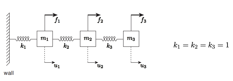
(a) original system \(A=\tilde{U}(k=0)\)

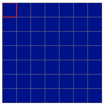
(b) processing pivot 1

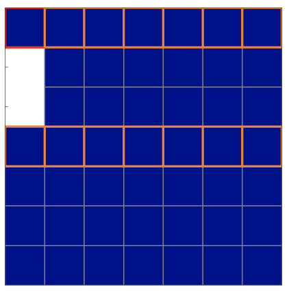
(c) beginning of step \(2, \tilde{U}(k=1)\)

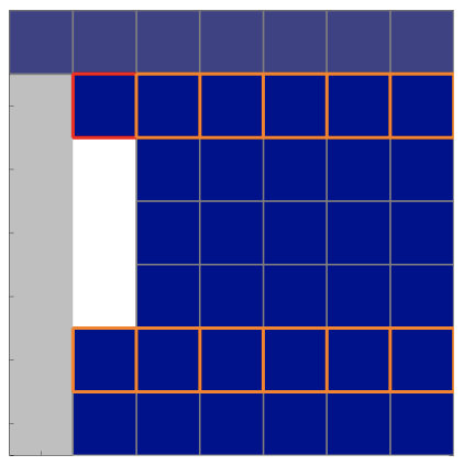
(d) processing pivot 2

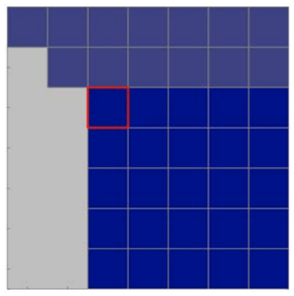
(e) beginning of step \(3, \tilde{U}(k=2)\)

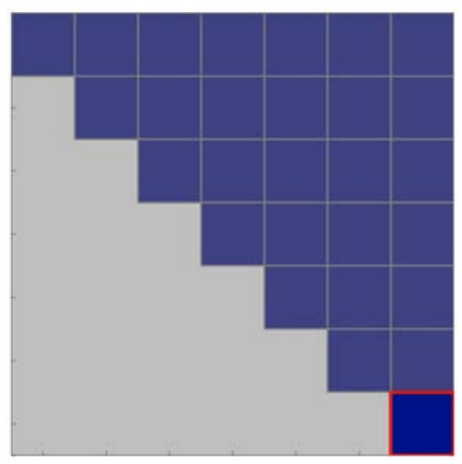
(f) final matrix \(U=\tilde{U}(k=n)\)

Figure 26.4: Illustration of Gaussian elimination applied to a \(6 \times 6\) system. See the main text for a description of the colors.