27.3: Gaussian Elimination and Back Substitution

Gaussian Elimination

We now consider the operation count associated with solving a sparse linear system \(A u=f\) using Gaussian elimination and back substitution introduced in the previous chapter. Recall that the Gaussian elimination is a process of turning a linear system into an upper triangular system, i.e. \[\operatorname{STEP} 1: A u=f \rightarrow \underset{\substack{(n \times n) \\ \text { upper } \\ \text { triangular }}}{U} \quad u=\hat{f}\] For a \(n \times n\) dense matrix, Gaussian elimination requires approximately \(\frac{2}{3} n^{3} \mathrm{FLOPs}^{\mathrm{S}}\).

Densely-Populated Banded Systems

Now, let us consider a \(n \times n\) banded matrix with a bandwidth \(m_{\mathrm{b}}\). To analyze the worst case, we assume that all entries within the band are nonzero. In the first step of Gaussian elimination, we identify the first row as the "pivot row" and eliminate the first entry (column 1) of the first \(m_{\mathrm{b}}\) rows by adding appropriately scaled pivot row; column 1 of rows \(m_{\mathrm{b}}+2, \ldots, n\) are already zero. Elimination of column 1 of a given row requires addition of scaled \(m_{\mathrm{b}}+1\) entries of the pivot row, which requires \(2\left(m_{\mathrm{b}}+1\right)\) operations. Applying the operation to \(m_{\mathrm{b}}\) rows, the operation count for the first step is approximately \(2\left(m_{\mathrm{b}}+1\right)^{2}\). Note that because the nonzero entries of the pivot row is confined to the first \(m_{\mathrm{b}}+1\) entries, addition of the scaled pivot row to the first \(m_{\mathrm{b}}+1\) rows does not increase the bandwidth of the system (since these rows already have nonzero entries in these columns). In particular, the sparsity pattern of the upper part of \(A\) is unaltered in the process.

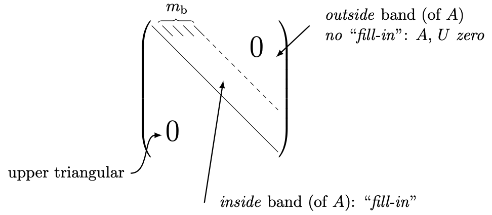
The second step of Gaussian elimination may be interpreted as applying the first step of Gaussian elimination to \((n-1) \times(n-1)\) submatrix, which itself is a banded matrix with a bandwidth \(m_{\mathrm{b}}\) (as the first step does not alter the bandwidth of the matrix). Thus, the second elimination step also requires approximately \(2\left(m_{\mathrm{b}}+1\right)^{2}\) FLOPs. Repeating the operation for all \(n\) pivots of the matrix, the total operation count for Gaussian elimination is approximately \(2 n\left(m_{\mathrm{b}}+1\right)^{2} \sim \mathcal{O}(n)\). The final upper triangular matrix \(U\) takes the following form:

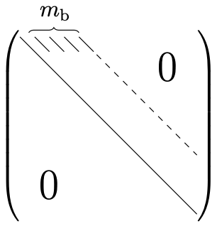
The upper triangular matrix has approximately \(n\left(m_{\mathrm{b}}+1\right) \sim \mathcal{O}(n)\) nonzero entries. Both the operation count and the number of nonzero in the final upper triangular matrix are \(\mathcal{O}(n)\), compared to \(\mathcal{O}\left(n^{3}\right)\) operations and \(\mathcal{O}\left(n^{2}\right)\) entries for a dense system. (We assume here \(m_{\mathrm{b}}\) is fixed independent of \(n\).)

In particular, as discussed in the previous chapter, Gaussian elimination of a tridiagonal matrix yields an upper bidiagonal matrix \[U=\left(\_{\text {main, main }+1 \text { diagonals }}^{0}\right.\] in approximately \(5 n\) operations (including the formation of the modified right-hand side \(\hat{f}\) ). Similarly, Gaussian elimination of a pentadiagonal system results in an upper triangular matrix of the form \[U=(\underbrace{0}_{\text {main, main }+1,+2 \text { diagonals }}\] and requires approximately \(14 n\) operations.

"Outrigger" Systems: Fill-Ins

Now let us consider application of Gaussian elimination to an "outrigger" system. First, because a \(n \times n\) "outrigger" system with a bandwidth \(m_{\mathrm{b}}\) is a special case of a "densely-populated banded" system with a bandwidth \(m_{\mathrm{b}}\) considered above, we know that the operation count for Gaussian elimination is at most \(n\left(m_{\mathrm{b}}+1\right)^{2}\) and the number of nonzero in the upper triangular matrix is at most \(n\left(m_{\mathrm{b}}+1\right)\). In addition, due to a large number of zero entries between the outer bands of the matrix, we hope that the operation count and the number of nonzero are less than those for the "densely-populated banded" case. Unfortunately, inspection of the Gaussian elimination procedure reveals that this reduction in the cost and storage is not achieved in general.

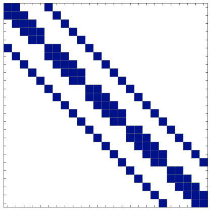
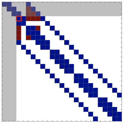
The inability to reduce the operation count is due to the introduction of "fill-ins": the entries of the sparse matrix that are originally zero but becomes nonzero in the Gaussian elimination process. The introduction of fill-ins is best described graphically. Figure \(\underline{27.3}\) shows a sequence of matrices generated through Gaussian elimination of a \(25 \times 25\) outrigger system. In the subsequent figures, we color code entries of partially processed \(U\) : the shaded area represents rows or columns of pivots already processed; the unshaded area represents the rows and columns of pivots not yet processed; the blue represent initial nonzeros in \(A\) which remain nonzeros in \(U\)-to-be; and the red are initial zeros of \(A\) which become nonzero in \(U\)-to-be, i.e. fill-ins.

As Figure 27.3(a) shows, the bandwidth of the original matrix is \(m_{\mathrm{b}}=5\). (The values of the entries are hidden in the figure as they are not important in this discussion of fill-ins.) In the first elimination step, we first eliminate column 1 of row 2 by adding an appropriately scaled row 1 to the row. While we succeed in eliminating column 1 of row 2 , note that we introduce a nonzero element in column 6 of row 2 as column 6 of row 1 "falls" to row 2 in the elimination process. This nonzero element is called a "fill-in." Similarly, in eliminating column 1 of row 6 , we introduce a "fill-in" in column 2 as column 2 of row 1 "falls" to row 6 in the elimination process. Thus, we have introduced two fill-ins in this first elimination step as shown in Figure 27.3(b): one in the upper part and another in the lower part.

Now, consider the second step of elimination starting from Figure 27.3(b). We first eliminate column 2 of row 3 by adding appropriately scaled row 2 to row 3 . This time, we introduce fill in not only from column 7 of row 2 "falling" to row 3, but also from column 6 of row 2 "falling" to row 3. Note that the latter is in fact a fill-in introduced in the first step. In general, once a fill-in is introduced in the upper part, the fill-in propagates from one step to the next, introducing further fill-ins as it "falls" through. Next, we need to eliminate column 2 of row 6 ; this entry was zero in the original matrix but was filled in the first elimination step. Thus, fill-in introduced in the lower part increases the number of rows whose leading entry must be eliminated in the upper-triangulation process. The matrix after the second step is shown in Figure 27.3(c). Note that the number of fill-in continue to increase, and we begin to lose the zero entries between the outer bands of the outrigger system.

As shown in Figure \(\underline{27.3(\mathrm{e})}\), by the beginning of the fifth elimination step, the "outrigger"

(a) original system \(A\)

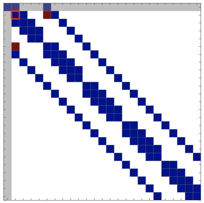
(b) beginning of step \(2, \tilde{U}(k=1)\)

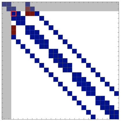
(c) beginning of step \(3, \tilde{U}(k=2)\)

(d) beginning of step \(4, \tilde{U}(k=3)\)

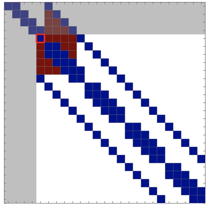
(e) beginning of step \(5, \tilde{U}(k=4)\)

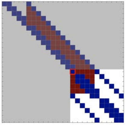
(f) beginning of step \(15, \tilde{U}(k=14)\)

Figure 27.3: Illustration of Gaussian elimination applied to a \(25 \times 25\) "outrigger" system. The blue entries are the entries present in the original system, and the red entries are "fill-in" introduced in the factorization process. The pivot for each step is marked by a red square.

system has largely lost its sparse structure in the leading \(\left(m_{\mathrm{b}}+1\right) \times\left(m_{\mathrm{b}}+1\right)\) subblock of the working submatrix. Thus, for the subsequent \(n-m_{\mathrm{b}}\) steps of Gaussian elimination, each step takes \(2 m_{\mathrm{b}}^{2}\) FLOPs, which is approximately the same number of operations as the densely-populated banded case. Thus, the total number of operations required for Gaussian elimination of an outrigger system is approximately \(2 n\left(m_{\mathrm{b}}+1\right)^{2}\), the same as the densely-populated banded case. The final matrix takes the form:

Note that the number of nonzero entries is approximately \(n\left(m_{\mathrm{b}}+1\right)\), which is much larger than the number of nonzero entries in the original "outrigger" system.

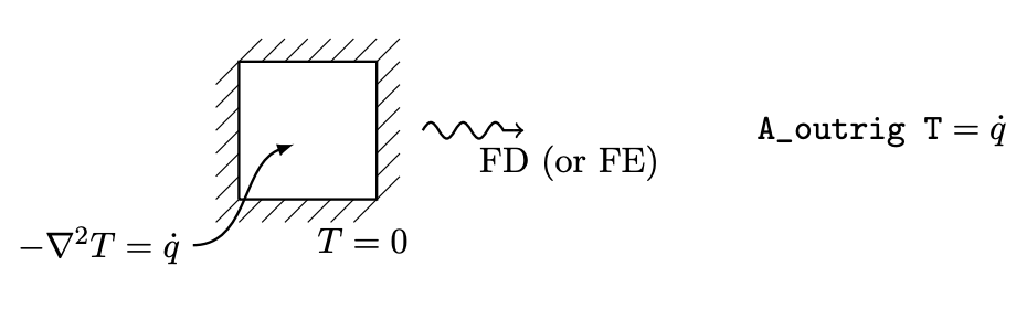
The "outrigger" system, such as the one considered above, naturally arise when a partial differential equation (PDE) is discretized in two or higher dimensions using a finite difference or finite element formulation. An example of such a PDE is the heat equation, describing, for example, the equilibrium temperature of a thermal system shown in Figure \(27.4\). With a natural ordering of the degrees of freedom of the discretized system, the bandwidth \(m_{\mathrm{b}}\) is equal to the number of grid points in one coordinate direction, and the number of degrees of freedom of the linear system is \(n=m_{\mathrm{b}}^{2}\) (i.e. product of the number of grid points in two coordinate directions). In other words, the bandwidth is the square root of the matrix size, i.e. \(m_{\mathrm{b}}=n^{1 / 2}\). Due to the outrigger structure of the resulting system, factorizing the system requires approximately \(n\left(m_{\mathrm{b}}+1\right)^{2} \approx n^{2}\) FLOPs. This is in contrast to one-dimensional case, which yields a tridiagonal system, which can be solved in \(\mathcal{O}(n)\) operations. In fact, in three dimensions, the bandwidth is equal to the product of the number of grid points in two coordinate directions, i.e. \(m_{\mathrm{b}}=\left(n^{1 / 3}\right)^{2}=n^{2 / 3}\). The number of operations required for factorization is \(n\left(m_{\mathrm{b}}+1\right)^{2} \approx n^{7 / 3}\). Thus, the cost of solving a PDE is significantly higher in three dimensions than in one dimension even if both discretized systems had the same number of unknowns. \({ }_{-}\)

Back Substitution

Having analyzed the operation count for Gaussian elimination, let us inspect the operation count for back substitution. First, recall that back substitution is a process of finding the solution of an upper triangular system, i.e. \[\text { STEP 2: } U u=\hat{f} \rightarrow u .\] Furthermore, recall that the operation count for back substitution is equal to twice the number of nonzero entries in \(U\). Because the matrix \(U\) is unaltered, we can simply count the number of

\({ }^{1}\) Not unknowns per dimension, but the total number of unknowns.

Figure 27.4: Heat equation in two dimensions. Discretization of the equation by finite difference (FD) or finite element (FE) method yields an "outrigger" system.

nonzero entries in the \(U\) that we obtain after Gaussian elimination; there is nothing equivalent to "fill-in" - modifications to the matrix that increases the number of entries in the matrix and hence the operation count - in back substitution.

Densely-Populated Banded Systems

For a densely-populated banded system with a bandwidth \(m_{\mathrm{b}}\), the number of unknowns in the factorized matrix \(U\) is approximately equal to \(n\left(m_{\mathrm{b}}+1\right)\). Thus, back substitution requires approximately \(2 n\left(m_{\mathrm{b}}+1\right)\) FLOPs. In particular, back substitution for a tridiagonal system (which yields an upper bidiagonal \(U\) ) requires approximately \(3 n\) FLOPs. A pentadiagonal system requires approximately \(5 n\) FLOPs.

"Outrigger"

As discussed above, a \(n \times n\) outrigger matrix of bandwidth \(m_{\mathrm{b}}\) produces an upper triangular matrix \(U\) whose entries between the main diagonal and the outer band are nonzero due to fill-ins. Thus, the number of nonzeros in \(U\) is approximately \(n\left(m_{\mathrm{b}}+1\right)\), and the operation count for back substitution is approximately \(2 n\left(m_{\mathrm{b}}+1\right)\). (Note in particular that even if an outrigger system only have five bands (as in the one shown in Figure \(27.3\) ), the number of operations for back substitution is \(2 n\left(m_{\mathrm{b}}+1\right)\) and not \(5 n\). \()\)