
27.4: Fill-in and Reordering
- Page ID
- 55707
\( \newcommand{\vecs}[1]{\overset { \scriptstyle \rightharpoonup} {\mathbf{#1}} } \)
\( \newcommand{\vecd}[1]{\overset{-\!-\!\rightharpoonup}{\vphantom{a}\smash {#1}}} \)
\( \newcommand{\dsum}{\displaystyle\sum\limits} \)
\( \newcommand{\dint}{\displaystyle\int\limits} \)
\( \newcommand{\dlim}{\displaystyle\lim\limits} \)
\( \newcommand{\id}{\mathrm{id}}\) \( \newcommand{\Span}{\mathrm{span}}\)
( \newcommand{\kernel}{\mathrm{null}\,}\) \( \newcommand{\range}{\mathrm{range}\,}\)
\( \newcommand{\RealPart}{\mathrm{Re}}\) \( \newcommand{\ImaginaryPart}{\mathrm{Im}}\)
\( \newcommand{\Argument}{\mathrm{Arg}}\) \( \newcommand{\norm}[1]{\| #1 \|}\)
\( \newcommand{\inner}[2]{\langle #1, #2 \rangle}\)
\( \newcommand{\Span}{\mathrm{span}}\)
\( \newcommand{\id}{\mathrm{id}}\)
\( \newcommand{\Span}{\mathrm{span}}\)
\( \newcommand{\kernel}{\mathrm{null}\,}\)
\( \newcommand{\range}{\mathrm{range}\,}\)
\( \newcommand{\RealPart}{\mathrm{Re}}\)
\( \newcommand{\ImaginaryPart}{\mathrm{Im}}\)
\( \newcommand{\Argument}{\mathrm{Arg}}\)
\( \newcommand{\norm}[1]{\| #1 \|}\)
\( \newcommand{\inner}[2]{\langle #1, #2 \rangle}\)
\( \newcommand{\Span}{\mathrm{span}}\) \( \newcommand{\AA}{\unicode[.8,0]{x212B}}\)
\( \newcommand{\vectorA}[1]{\vec{#1}} % arrow\)
\( \newcommand{\vectorAt}[1]{\vec{\text{#1}}} % arrow\)
\( \newcommand{\vectorB}[1]{\overset { \scriptstyle \rightharpoonup} {\mathbf{#1}} } \)
\( \newcommand{\vectorC}[1]{\textbf{#1}} \)
\( \newcommand{\vectorD}[1]{\overrightarrow{#1}} \)
\( \newcommand{\vectorDt}[1]{\overrightarrow{\text{#1}}} \)
\( \newcommand{\vectE}[1]{\overset{-\!-\!\rightharpoonup}{\vphantom{a}\smash{\mathbf {#1}}}} \)
\( \newcommand{\vecs}[1]{\overset { \scriptstyle \rightharpoonup} {\mathbf{#1}} } \)
\(\newcommand{\longvect}{\overrightarrow}\)
\( \newcommand{\vecd}[1]{\overset{-\!-\!\rightharpoonup}{\vphantom{a}\smash {#1}}} \)
\(\newcommand{\avec}{\mathbf a}\) \(\newcommand{\bvec}{\mathbf b}\) \(\newcommand{\cvec}{\mathbf c}\) \(\newcommand{\dvec}{\mathbf d}\) \(\newcommand{\dtil}{\widetilde{\mathbf d}}\) \(\newcommand{\evec}{\mathbf e}\) \(\newcommand{\fvec}{\mathbf f}\) \(\newcommand{\nvec}{\mathbf n}\) \(\newcommand{\pvec}{\mathbf p}\) \(\newcommand{\qvec}{\mathbf q}\) \(\newcommand{\svec}{\mathbf s}\) \(\newcommand{\tvec}{\mathbf t}\) \(\newcommand{\uvec}{\mathbf u}\) \(\newcommand{\vvec}{\mathbf v}\) \(\newcommand{\wvec}{\mathbf w}\) \(\newcommand{\xvec}{\mathbf x}\) \(\newcommand{\yvec}{\mathbf y}\) \(\newcommand{\zvec}{\mathbf z}\) \(\newcommand{\rvec}{\mathbf r}\) \(\newcommand{\mvec}{\mathbf m}\) \(\newcommand{\zerovec}{\mathbf 0}\) \(\newcommand{\onevec}{\mathbf 1}\) \(\newcommand{\real}{\mathbb R}\) \(\newcommand{\twovec}[2]{\left[\begin{array}{r}#1 \\ #2 \end{array}\right]}\) \(\newcommand{\ctwovec}[2]{\left[\begin{array}{c}#1 \\ #2 \end{array}\right]}\) \(\newcommand{\threevec}[3]{\left[\begin{array}{r}#1 \\ #2 \\ #3 \end{array}\right]}\) \(\newcommand{\cthreevec}[3]{\left[\begin{array}{c}#1 \\ #2 \\ #3 \end{array}\right]}\) \(\newcommand{\fourvec}[4]{\left[\begin{array}{r}#1 \\ #2 \\ #3 \\ #4 \end{array}\right]}\) \(\newcommand{\cfourvec}[4]{\left[\begin{array}{c}#1 \\ #2 \\ #3 \\ #4 \end{array}\right]}\) \(\newcommand{\fivevec}[5]{\left[\begin{array}{r}#1 \\ #2 \\ #3 \\ #4 \\ #5 \\ \end{array}\right]}\) \(\newcommand{\cfivevec}[5]{\left[\begin{array}{c}#1 \\ #2 \\ #3 \\ #4 \\ #5 \\ \end{array}\right]}\) \(\newcommand{\mattwo}[4]{\left[\begin{array}{rr}#1 \amp #2 \\ #3 \amp #4 \\ \end{array}\right]}\) \(\newcommand{\laspan}[1]{\text{Span}\{#1\}}\) \(\newcommand{\bcal}{\cal B}\) \(\newcommand{\ccal}{\cal C}\) \(\newcommand{\scal}{\cal S}\) \(\newcommand{\wcal}{\cal W}\) \(\newcommand{\ecal}{\cal E}\) \(\newcommand{\coords}[2]{\left\{#1\right\}_{#2}}\) \(\newcommand{\gray}[1]{\color{gray}{#1}}\) \(\newcommand{\lgray}[1]{\color{lightgray}{#1}}\) \(\newcommand{\rank}{\operatorname{rank}}\) \(\newcommand{\row}{\text{Row}}\) \(\newcommand{\col}{\text{Col}}\) \(\renewcommand{\row}{\text{Row}}\) \(\newcommand{\nul}{\text{Nul}}\) \(\newcommand{\var}{\text{Var}}\) \(\newcommand{\corr}{\text{corr}}\) \(\newcommand{\len}[1]{\left|#1\right|}\) \(\newcommand{\bbar}{\overline{\bvec}}\) \(\newcommand{\bhat}{\widehat{\bvec}}\) \(\newcommand{\bperp}{\bvec^\perp}\) \(\newcommand{\xhat}{\widehat{\xvec}}\) \(\newcommand{\vhat}{\widehat{\vvec}}\) \(\newcommand{\uhat}{\widehat{\uvec}}\) \(\newcommand{\what}{\widehat{\wvec}}\) \(\newcommand{\Sighat}{\widehat{\Sigma}}\) \(\newcommand{\lt}{<}\) \(\newcommand{\gt}{>}\) \(\newcommand{\amp}{&}\) \(\definecolor{fillinmathshade}{gray}{0.9}\)Begin Advanced Material
The previous section focused on the computational cost of solving a linear system governed by banded sparse matrices. This section introduces a few additional sparse matrices and also discussed additional concepts on Gaussian elimination for sparse systems.
Cyclic System
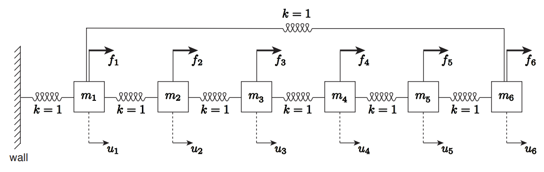
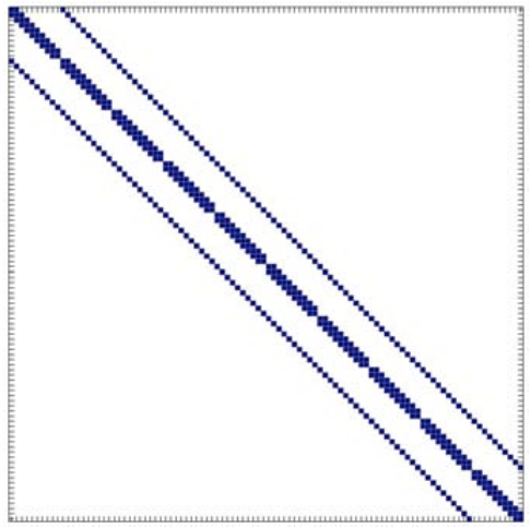
First, let us show that a small change in a physical system - and hence the corresponding linear system \(A\) - can make a large difference in the sparsity pattern of the factored matrix \(U\). Here, we consider a modified version of \(n\)-mass mass-spring system, where the first mass is connected to the last mass, as shown in Figure 27.5. We will refer to this system as a "cyclic" system, as the springs form a circle. Recall that a spring-mass system without the extra connection yields a tridiagonal system. With the extra connection between the first and the last mass, now the \((1, n)\) entry and \((n, 1)\) entry of the matrix are nonzero as shown in Figure \(27.6(\mathrm{a})\) (for \(n=25\) ); clearly, the matrix
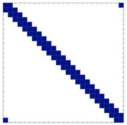
(a) original matrix \(A\)
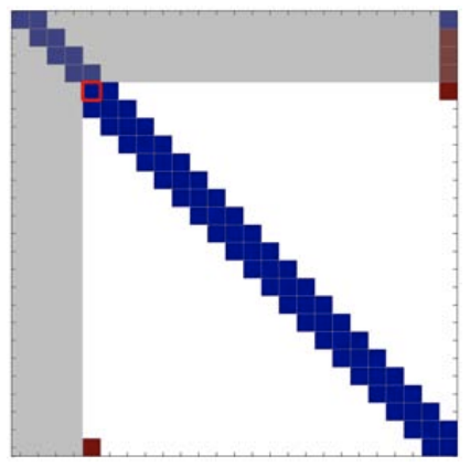
(b) beginning of step 5
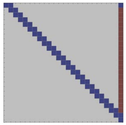
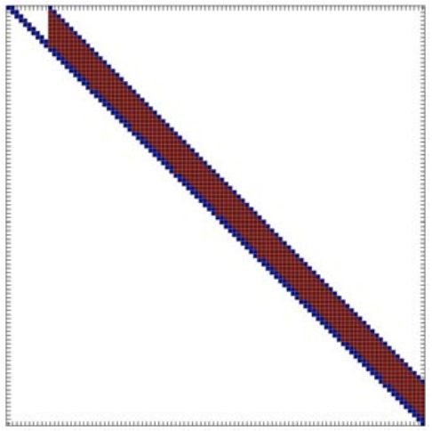
(c) final matrix \(U\)
Figure 27.6: Illustration of Gaussian elimination applied to a \(25 \times 25\) "arrow" system. The red entries are "fill-in" introduced in the factorization process. The pivot for each step is marked by a red square.
is no longer tridiagonal. In fact, if apply our standard classification for banded matrices, the cyclic matrix would be characterized by its bandwidth of \(m_{\mathrm{b}}=n-1\).
Applying Gaussian elimination to the "cyclic" system, we immediately recognize that the \((1, n)\) entry of the original matrix "falls" along the last column, creating \(n-2\) fill-ins (see Figures \(27.6(\mathrm{~b})\) and \(27.6(\mathrm{c}))\). In addition, the original \((n, 1)\) entry also creates a nonzero entry on the bottom row, which moves across the matrix with the pivot as the matrix is factorized. As a result, the operation count for the factorization of the "cyclic" system is in fact similar to that of a pentadiagonal system: approximately \(14 n\) FLOPs. Applying back substitution to the factored matrix - which contains approximately \(3 n\) nonzeros - require \(5 n\) FLOPs. Thus, solution of the cyclic system - which has just two more nonzero entries than the tridiagonal system - requires more than twice the operations \((19 n\) vs. \(8 n)\). However, it is also important to note that this \(\mathcal{O}(n)\) operation count is a significant improvement compared to the \(\mathcal{O}\left(n\left(m_{\mathrm{b}}+1\right)^{2}\right)=\mathcal{O}\left(n^{3}\right)\) operation estimate based on classifying the system as a standard "outrigger" with a bandwidth \(m_{\mathrm{b}}=n-1\).
We note that the fill-in structure of \(U\) takes the form of a skyline defined by the envelope of the columns of the original matrix \(A\). This is a general principal.
Reordering
In constructing a linear system corresponding to our spring-mass system, we associated the \(j^{\text {th }}\) entry of the solution vector - and hence the \(j^{\text {th }}\) column of the matrix - with the displacement of the \(j^{\text {th }}\) mass (counting from the wall) and associated the \(i^{\text {th }}\) equation with the force equilibrium condition
(a) \(A\) (natural, \(\mathrm{nnz}(A)=460)\)
(b) \(U\) (natural, \(\operatorname{nnz}(U)=1009\) )
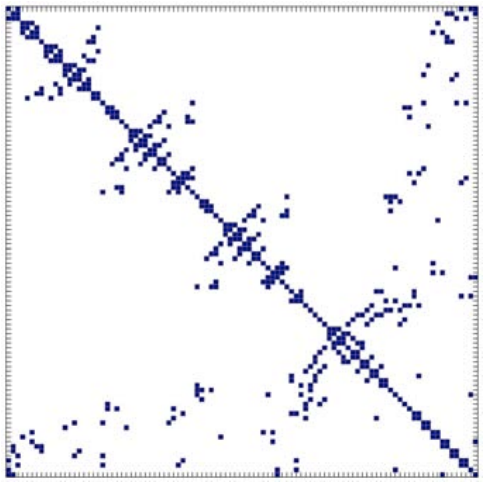
(c) \(A^{\prime}\left(\mathrm{AMD}, \operatorname{nnz}\left(A^{\prime}\right)=460\right)\)
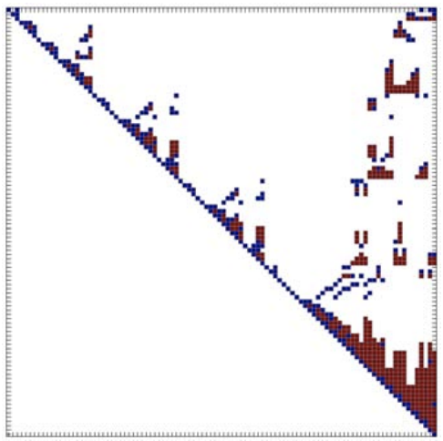
(d) \(U^{\prime}\left(\mathrm{AMD}, \mathrm{nnz}\left(U^{\prime}\right)=657\right)\)
Figure 27.7: Comparison of the sparsity pattern and Gaussian elimination fill-ins for a \(n=100\) "outrigger" system resulting from natural ordering and an equivalent system using the approximate minimum degree (AMD) ordering.
of the \(i^{\text {th }}\) mass. While this is arguably the most "natural" ordering for the spring-mass system, we could have associated a given column and row of the matrix with a different displacement and force equilibrium condition, respectively. Note that this "reordering" of the unknowns and equations of the linear system is equivalent to "swapping" the rows of columns of the matrix, which is formally known as permutation. Importantly, we can describe the same physical system using many different orderings of the unknowns and equations; even if the matrices appear different, these matrices describing the same physical system may be considered equivalent, as they all produce the same solution for a given right-hand side (given both the solution and right-hand side are reordered in a consistent manner).
Reordering can make a significant difference in the number of fill-ins and the operation count. Figure \(27.7\) shows a comparison of number of fill-ins for an \(n=100\) linear system arising from two different orderings of a finite different discretization of two-dimensional heat equation on a \(10 \times 10\) computational grid. An "outrigger" matrix of bandwidth \(m_{\mathrm{b}}=10\) arising from "natural" ordering is shown in Figure 27.7(a). The matrix has 460 nonzero entries. As discussed in the previous section, Gaussian elimination of the matrix yields an upper triangular matrix \(U\) with approximately \(n\left(m_{\mathrm{b}}+1\right)=1100\) nonzero entries (more precisely 1009 for this particular case), which is shown in Figure 27.7(b). An equivalent system obtained using the approximate minimum degree (AMD) ordering is shown in Figure 27.7(c). This newly reordered matrix \(A^{\prime}\) also has 460 nonzero entries because permuting (or swapping) rows and columns clearly does not change the number of nonzeros. On the other hand, application of Gaussian elimination to this reordered matrix yields an upper triangular matrix \(U\) shown in Figure \(27.7(\mathrm{~d})\), which has only 657 nonzero entries. Note that the number of fill-in has been reduced by roughly a factor of two: from \(1009-280=729\) for the "natural" ordering to \(657-280=377\) for the AMD ordering. (The original matrix \(A\) has 280 nonzero entries in the upper triangular part.)
In general, using an appropriate ordering can significantly reduced the number of fill-ins and hence the computational cost. In particular, for a sparse matrix arising from \(n\)-unknown finite difference (or finite element) discretization of two-dimensional PDEs, we have noted that "natural" ordering produces an "outrigger" system with \(m_{\mathrm{b}}=\sqrt{n}\); Gaussian elimination of the system yields an upper triangular matrix with \(n\left(m_{\mathrm{b}}+1\right) \approx n^{3 / 2}\) nonzero entries. On the other hand, the number of fill-ins for the same system with an optimal (i.e. minimum fill-in) ordering yields an upper triangular matrix with \(\mathcal{O}(n \log (n))\) unknowns. Thus, ordering can have significant impact in both the operation count and storage for large sparse linear systems.