27.5: The Evil Inverse

In solving a linear system \(A u=f\), we advocated a two-step strategy that consists of Gaussian elimination and back substitution, i.e. \[\begin{aligned} \text { Gaussian elimination: } & A u=f \quad \Rightarrow \quad U u=\hat{f} \\ \text { Back substitution: } & U u=\hat{f} \quad \Rightarrow \quad u . \end{aligned}\] Alternatively, we could find \(u\) by explicitly forming the inverse of \(A, A^{-1}\). Recall that if \(A\) is nonsingular (as indicated by, for example, independent columns), there exists a unique matrix \(A^{-1}\) such that \[A A^{-1}=I \text { and } A^{-1} A=I .\] The inverse matrix \(A^{-1}\) is relevant to solution systems because, in principle, we could

1. Construct \(A^{-1}\);
2. Evaluate \(u=A^{-1} f\) (i.e. matrix-vector product).

Note that the second step follows from the fact that \[\begin{aligned} A u &=f \\ A^{-1} A u &=A^{-1} f \\ I u &=A^{-1} f . \end{aligned}\] While the procedure is mathematically valid, we warn that a linear system should never be solved by explicitly forming the inverse.

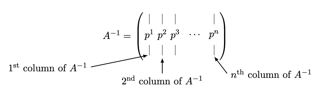
To motivate why explicitly construction of inverse matrices should be avoided, let us study the sparsity pattern of the inverse matrix for a \(n\)-mass spring-mass system, an example of which for \(n=5\) is shown in Figure \(27.8\). We use the column interpretation of the matrix and associate the column \(j\) of \(A^{-1}\) with a vector \(p^{j}\), i.e.

Figure 27.8: Response of a \(n=5\) spring-mass system to unit loading on mass 3.

Since \(A u=f\) and \(u=A^{-1} f\), we have (using one-handed matrix-vector product),

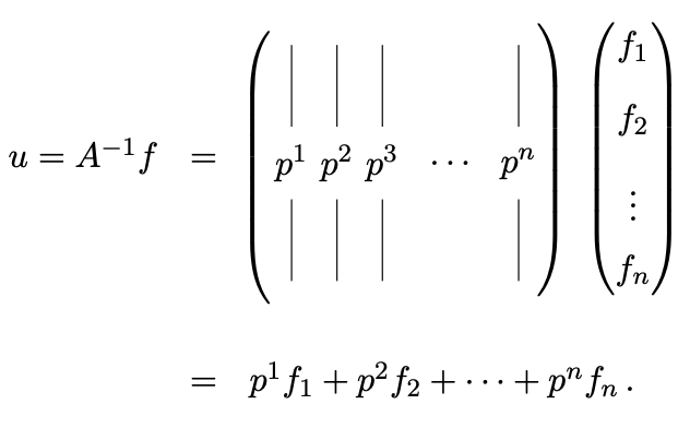
From this expression, it is clear that the vector \(p^{j}\) is equal to the displacements of masses due to the unit force acting on mass \(j\). In particular the \(i^{\text {th }}\) entry of \(p^{j}\) is the displacement of the \(i^{\text {th }}\) mass due to the unit force on the \(j^{\text {th }}\) mass.

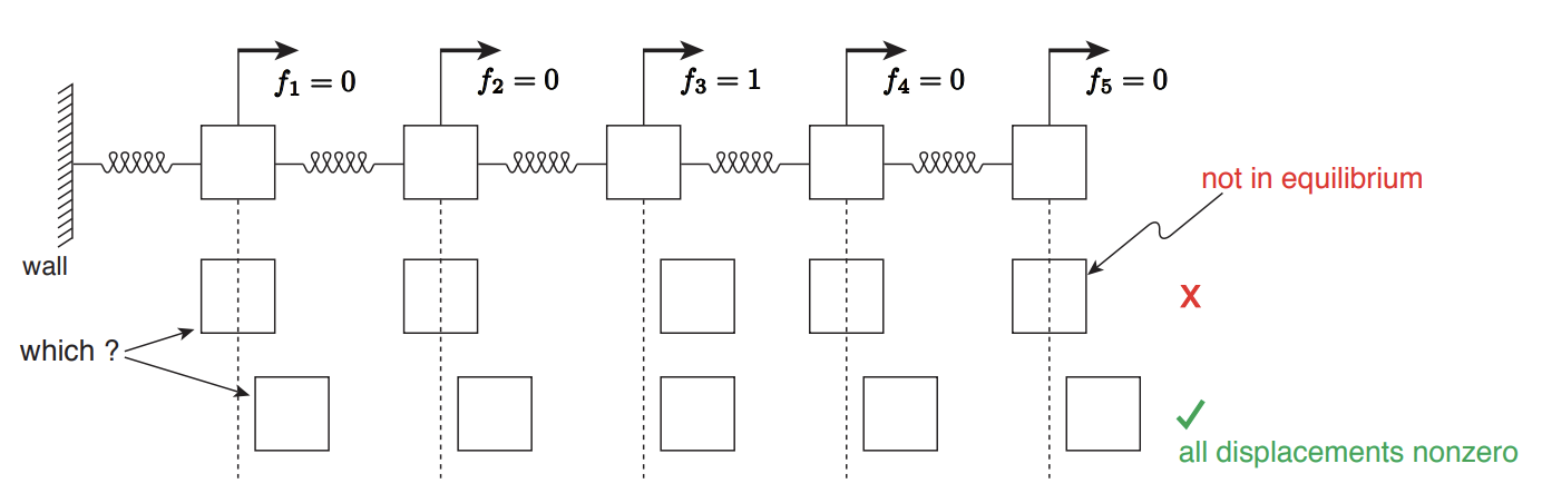
Now, to deduce nonzero pattern of a vector \(p^{j}\), let us focus on the case shown in Figure \(27.8\); we will deduce the nonzero entries of \(p^{3}\) for the \(n=5\) system. Let us consider a sequence of events that takes place when \(f_{3}\) is applied (we focus on qualitative result rather than quantitative result, i.e. whether masses move, not by how much):

1. Mass 3 moves to the right due to the unit load \(f_{3}\).
2. Force exerted by the spring connecting mass 3 and 4 increases as the distance between mass 3 and 4 decreases.
3. Mass 4 is no longer in equilibrium as there is a larger force from the left than from the right (i.e. from the spring connecting mass 3 and 4, which is now compressed, than from the spring connecting mass 4 and 5 , which is neutral). 4. Due to the unbalanced force mass 4 moves to the right.
4. The movement of mass 4 to the left triggers a sequence of event that moves mass 5 , just as the movement of mass 3 displaced mass 4. Namely, the force on the spring connecting mass 4 and 5 increases, mass 5 is no longer in equilibrium, and mass 5 moves to the right.

Thus, it is clear that the unit load on mass 3 not only moves mass 3 but also mass 4 and 5 in Figure \(27.8\). Using the same qualitative argument, we can convince ourselves that mass 1 and 2 must also move when mass 3 is displaced by the unit load. Thus, in general, the unit load \(f_{3}\) on mass 3 results in displacing all masses of the system. Recalling that the \(i^{\text {th }}\) entry of \(p^{3}\) is the displacement of the \(i^{\text {th }}\) mass due to the unit load \(f_{3}\), we conclude that all entries of \(p^{3}\) are nonzero. (In absence of damping, the system excited by the unit load would oscillate and never come to rest; in a real system, intrinsic damping present in the springs brings the system to a new equilibrium state.)

Generalization of the above argument to a \(n\)-mass system is straightforward. Furthermore, using the same argument, we conclude that forcing of any of one of the masses results in displacing all masses. Consequently, for \(p^{1}, \ldots, p^{n}\), we have

Recalling that \(p^{j}\) is the \(j^{\text {th }}\) column of \(A^{-1}\), we conclude that \[A^{-1}=\left(\begin{array}{llll} & & & \\ p^{1} & p^{2} & \cdots & p^{n} \end{array}\right)\] is full even though (here) \(A\) is tridiagonal. In general \(A^{-1}\) does not preserve sparsity of \(A\) and is in fact often full. This is unlike the upper triangular matrix resulting from Gaussian elimination, which preserves a large number of zeros (modulo the fill-ins).

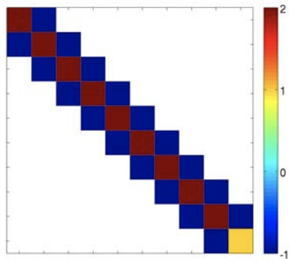
Figure \(27.9\) shows the system matrix and its inverse for the \(n=10\) spring-mass system. The colors represent the value of each entries; for instance, the \(A\) matrix has the typical \(\left[\begin{array}{ccc}-1 & 2 & -1\end{array}\right]\) pattern, except for the first and last equations. Note that the inverse matrix is not sparse and is in fact full. In addition, the values of each column of \(A^{-1}\) agrees with our physical intuition about the displacements to a unit load. For example, when a unit load is applied to mass 3 , the distance between the wall and mass 1 increases by 1 unit, the distance between mass 1 and 2 increases by 1 unit, and the distance between mass 3 and 2 increases by 1 unit; the distances between the remaining masses are unaltered because there is no external force acting on the remaining system at equilibrium (because our system is not clamped on the right end). Accumulating displacements starting with mass 1 , we conclude that mass 1 moves by 1 , mass 2 moves by 2 (the sum of the increased distances between mass 1 and 2 and mass 2 and 3), mass 3 moves by 3 , and all the remaining masses move by 3 . This is exactly the information contained in the third column of \(A^{-1}\), which reads \(\left[\begin{array}{llllll}1 & 2 & 3 & 3 & \ldots & 3\end{array}\right]^{\mathrm{T}}\).

In concluding the section, let us analyze the operation count for solving a linear system by explicitly forming the inverse and performing matrix-vector multiplication. We assume that our \(n \times n\) matrix \(A\) has a bandwidth of \(m_{\mathrm{b}}\). First, we construct the inverse matrix one column at a time \[\begin{aligned} & u\left[\text { for } f=\left(\begin{array}{llll}1 & 0 & \cdots & 0\end{array}\right)^{\mathrm{T}}\right]=p^{1} \leftarrow \text { nonzero in all entries! } \\ & u\left[\text { for } f=\left(\begin{array}{llll}0 & 1 & \cdots & 0\end{array}\right)^{\mathrm{T}}\right]=p^{2} \leftarrow \text { nonzero in all entries! } \\ & u\left[\text { for } f=\left(\begin{array}{llll}0 & 0 & \cdots & 0\end{array}\right)^{\mathrm{T}}\right]=p^{n} \leftarrow \text { nonzero in all entries! } \end{aligned}\]

(a) \(A\)

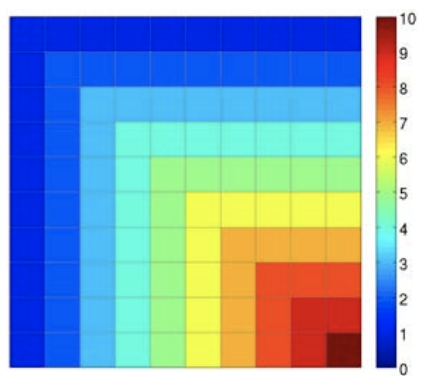
(b) \(A^{-1}\)

Figure 27.9: Matrix \(A\) for the \(n=10\) spring-mass system and its inverse \(A^{-1}\). The colors represent the value of each entry as specified by the color bar.

by solving for the equilibrium displacements associated with unit load on each mass. To this end, we first compute the LU factorization of \(A\) and then repeat forward/backward substitution. Recalling the operation count for a single forward/backward substitution is \(\mathcal{O}\left(n m_{\mathrm{b}}^{2}\right)\), the construction of \(A^{-1}\) requires \[\begin{aligned} A p^{1}=&\left(\begin{array}{c} 1 \\ 0 \\ \vdots \\ 0 \end{array}\right) \Rightarrow p^{1} \quad \mathcal{O}\left(n m_{\mathrm{b}}^{2}\right) \mathrm{FLOPs} \\ & \vdots \\ A p^{n} &=\left(\begin{array}{c} 0 \\ 0 \\ \vdots \\ 1 \end{array}\right) \Rightarrow p^{n} \quad \mathcal{O}\left(n m_{\mathrm{b}}^{2}\right) \mathrm{FLOPs} \end{aligned}\] for the total work of \(n \cdot \mathcal{O}\left(n m_{\mathrm{b}}^{2}\right) \sim \mathcal{O}\left(n^{2} m_{\mathrm{b}}^{2}\right)\) FLOPs. Once we formed the inverse matrix, we can solve for the displacement by performing (dense) matrix-vector multiplication, i.e. \[\left(\begin{array}{c} u_{1} \\ u_{2} \\ \vdots \\ u_{n} \end{array}\right)=\left(\begin{array}{cccc} \times & x & \cdots & \times \\ \times & \times & \cdots & \times \\ \vdots & \vdots & \ddots & \vdots \\ \times & \times & \cdots & \times \\ A^{-1} & (\text { full }) & \mathcal{O}(n \cdot n)=\mathcal{O}\left(n^{2}\right) \mathrm{FLOPs} \\ f_{n} \end{array}\right) \quad \text { one-handed or two-handed }\] Thus, both the construction of the inverse matrix and the matrix-vector multiplication require \(\mathcal{O}\left(n^{2}\right)\) operations. In contrast recall that Gaussian elimination and back substitution solves a sparse linear system in \(\mathcal{O}(n)\) operations. Thus, a large sparse linear system should never be solved by explicitly forming its inverse.