
29.1: Introduction
- Page ID
- 55712
\( \newcommand{\vecs}[1]{\overset { \scriptstyle \rightharpoonup} {\mathbf{#1}} } \)
\( \newcommand{\vecd}[1]{\overset{-\!-\!\rightharpoonup}{\vphantom{a}\smash {#1}}} \)
\( \newcommand{\dsum}{\displaystyle\sum\limits} \)
\( \newcommand{\dint}{\displaystyle\int\limits} \)
\( \newcommand{\dlim}{\displaystyle\lim\limits} \)
\( \newcommand{\id}{\mathrm{id}}\) \( \newcommand{\Span}{\mathrm{span}}\)
( \newcommand{\kernel}{\mathrm{null}\,}\) \( \newcommand{\range}{\mathrm{range}\,}\)
\( \newcommand{\RealPart}{\mathrm{Re}}\) \( \newcommand{\ImaginaryPart}{\mathrm{Im}}\)
\( \newcommand{\Argument}{\mathrm{Arg}}\) \( \newcommand{\norm}[1]{\| #1 \|}\)
\( \newcommand{\inner}[2]{\langle #1, #2 \rangle}\)
\( \newcommand{\Span}{\mathrm{span}}\)
\( \newcommand{\id}{\mathrm{id}}\)
\( \newcommand{\Span}{\mathrm{span}}\)
\( \newcommand{\kernel}{\mathrm{null}\,}\)
\( \newcommand{\range}{\mathrm{range}\,}\)
\( \newcommand{\RealPart}{\mathrm{Re}}\)
\( \newcommand{\ImaginaryPart}{\mathrm{Im}}\)
\( \newcommand{\Argument}{\mathrm{Arg}}\)
\( \newcommand{\norm}[1]{\| #1 \|}\)
\( \newcommand{\inner}[2]{\langle #1, #2 \rangle}\)
\( \newcommand{\Span}{\mathrm{span}}\) \( \newcommand{\AA}{\unicode[.8,0]{x212B}}\)
\( \newcommand{\vectorA}[1]{\vec{#1}} % arrow\)
\( \newcommand{\vectorAt}[1]{\vec{\text{#1}}} % arrow\)
\( \newcommand{\vectorB}[1]{\overset { \scriptstyle \rightharpoonup} {\mathbf{#1}} } \)
\( \newcommand{\vectorC}[1]{\textbf{#1}} \)
\( \newcommand{\vectorD}[1]{\overrightarrow{#1}} \)
\( \newcommand{\vectorDt}[1]{\overrightarrow{\text{#1}}} \)
\( \newcommand{\vectE}[1]{\overset{-\!-\!\rightharpoonup}{\vphantom{a}\smash{\mathbf {#1}}}} \)
\( \newcommand{\vecs}[1]{\overset { \scriptstyle \rightharpoonup} {\mathbf{#1}} } \)
\(\newcommand{\longvect}{\overrightarrow}\)
\( \newcommand{\vecd}[1]{\overset{-\!-\!\rightharpoonup}{\vphantom{a}\smash {#1}}} \)
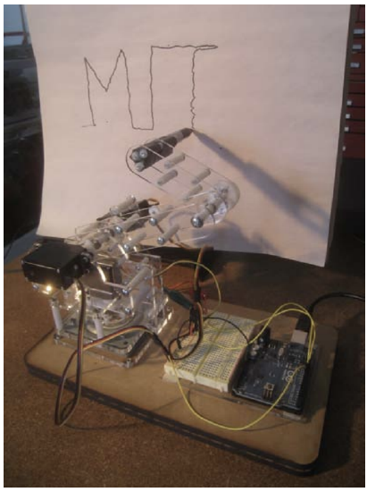
\(\newcommand{\avec}{\mathbf a}\) \(\newcommand{\bvec}{\mathbf b}\) \(\newcommand{\cvec}{\mathbf c}\) \(\newcommand{\dvec}{\mathbf d}\) \(\newcommand{\dtil}{\widetilde{\mathbf d}}\) \(\newcommand{\evec}{\mathbf e}\) \(\newcommand{\fvec}{\mathbf f}\) \(\newcommand{\nvec}{\mathbf n}\) \(\newcommand{\pvec}{\mathbf p}\) \(\newcommand{\qvec}{\mathbf q}\) \(\newcommand{\svec}{\mathbf s}\) \(\newcommand{\tvec}{\mathbf t}\) \(\newcommand{\uvec}{\mathbf u}\) \(\newcommand{\vvec}{\mathbf v}\) \(\newcommand{\wvec}{\mathbf w}\) \(\newcommand{\xvec}{\mathbf x}\) \(\newcommand{\yvec}{\mathbf y}\) \(\newcommand{\zvec}{\mathbf z}\) \(\newcommand{\rvec}{\mathbf r}\) \(\newcommand{\mvec}{\mathbf m}\) \(\newcommand{\zerovec}{\mathbf 0}\) \(\newcommand{\onevec}{\mathbf 1}\) \(\newcommand{\real}{\mathbb R}\) \(\newcommand{\twovec}[2]{\left[\begin{array}{r}#1 \\ #2 \end{array}\right]}\) \(\newcommand{\ctwovec}[2]{\left[\begin{array}{c}#1 \\ #2 \end{array}\right]}\) \(\newcommand{\threevec}[3]{\left[\begin{array}{r}#1 \\ #2 \\ #3 \end{array}\right]}\) \(\newcommand{\cthreevec}[3]{\left[\begin{array}{c}#1 \\ #2 \\ #3 \end{array}\right]}\) \(\newcommand{\fourvec}[4]{\left[\begin{array}{r}#1 \\ #2 \\ #3 \\ #4 \end{array}\right]}\) \(\newcommand{\cfourvec}[4]{\left[\begin{array}{c}#1 \\ #2 \\ #3 \\ #4 \end{array}\right]}\) \(\newcommand{\fivevec}[5]{\left[\begin{array}{r}#1 \\ #2 \\ #3 \\ #4 \\ #5 \\ \end{array}\right]}\) \(\newcommand{\cfivevec}[5]{\left[\begin{array}{c}#1 \\ #2 \\ #3 \\ #4 \\ #5 \\ \end{array}\right]}\) \(\newcommand{\mattwo}[4]{\left[\begin{array}{rr}#1 \amp #2 \\ #3 \amp #4 \\ \end{array}\right]}\) \(\newcommand{\laspan}[1]{\text{Span}\{#1\}}\) \(\newcommand{\bcal}{\cal B}\) \(\newcommand{\ccal}{\cal C}\) \(\newcommand{\scal}{\cal S}\) \(\newcommand{\wcal}{\cal W}\) \(\newcommand{\ecal}{\cal E}\) \(\newcommand{\coords}[2]{\left\{#1\right\}_{#2}}\) \(\newcommand{\gray}[1]{\color{gray}{#1}}\) \(\newcommand{\lgray}[1]{\color{lightgray}{#1}}\) \(\newcommand{\rank}{\operatorname{rank}}\) \(\newcommand{\row}{\text{Row}}\) \(\newcommand{\col}{\text{Col}}\) \(\renewcommand{\row}{\text{Row}}\) \(\newcommand{\nul}{\text{Nul}}\) \(\newcommand{\var}{\text{Var}}\) \(\newcommand{\corr}{\text{corr}}\) \(\newcommand{\len}[1]{\left|#1\right|}\) \(\newcommand{\bbar}{\overline{\bvec}}\) \(\newcommand{\bhat}{\widehat{\bvec}}\) \(\newcommand{\bperp}{\bvec^\perp}\) \(\newcommand{\xhat}{\widehat{\xvec}}\) \(\newcommand{\vhat}{\widehat{\vvec}}\) \(\newcommand{\uhat}{\widehat{\uvec}}\) \(\newcommand{\what}{\widehat{\wvec}}\) \(\newcommand{\Sighat}{\widehat{\Sigma}}\) \(\newcommand{\lt}{<}\) \(\newcommand{\gt}{>}\) \(\newcommand{\amp}{&}\) \(\definecolor{fillinmathshade}{gray}{0.9}\)The demonstration robot arm of Figure \(29.1\) is represented schematically in Figure 29.2. Note that although the robot of Figure \(29.1\) has three degrees-of-freedom ( "shoulder," "elbow," and "waist"), we will be dealing with only two degrees-of-freedom - "shoulder" and "elbow" - in this assignment.
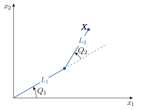
The forward kinematics of the robot arm determine the coordinates of the end effector \(\boldsymbol{X}=\) \(\left[X_{1}, X_{2}\right]^{\mathrm{T}}\) for given joint angles \(\boldsymbol{Q}=\left[Q_{1}, Q_{2}\right]^{\mathrm{T}}\) as \[\left[\begin{array}{l} X_{1} \\ X_{2} \end{array}\right](\boldsymbol{Q})=\left[\begin{array}{c} L_{1} \cos \left(Q_{1}\right)+L_{2} \cos \left(Q_{1}+Q_{2}\right) \\ L_{1} \sin \left(Q_{1}\right)+L_{2} \sin \left(Q_{1}+Q_{2}\right) \end{array}\right],\] where \(L_{1}\) and \(L_{2}\) are the lengths of the first and second arm links, respectively. For our robot, \(L_{1}=4\) inches and \(L_{2}=3.025\) inches.
The inverse kinematics of the robot arm - the joint angles \(\boldsymbol{Q}\) needed to realize a particular end effector position \(\boldsymbol{X}\) - are not so straightforward and, for many more complex robot arms, a closed-form solution does not exist. In this assignment, we will solve the inverse kinematic problem for a two degree-of-freedom, planar robot arm by solving numerically for \(Q_{1}\) and \(Q_{2}\) from the set of nonlinear Equations (29.1) .
Given a trajectory of data vectors \(\boldsymbol{X}_{(i)}, 1 \leq i \leq p\) - a sequence of \(p\) desired end effector positions - the corresponding joint angles satisfy \[\boldsymbol{F}\left(\boldsymbol{Q}_{(i)}, \boldsymbol{X}_{(i))}=0, \quad 1 \leq i \leq p,\right.\] where \[\boldsymbol{F}(\boldsymbol{q}, \boldsymbol{X})=\left[\begin{array}{l} F_{1} \\ F_{2} \end{array}\right]=\left[\begin{array}{c} L_{1} \cos \left(q_{1}\right)+L_{2} \cos \left(q_{1}+q_{2}\right)-X_{1} \\ L_{1} \sin \left(q_{1}\right)+L_{2} \sin \left(q_{1}+q_{2}\right)-X_{2} \end{array}\right]\] For the robot "home" position, \(\boldsymbol{X}^{\text {home }} \approx[-0.7154,6.9635]^{\mathrm{T}}\), the joint angles are known: \(\boldsymbol{Q}^{\text {home }}=\) \([1.6,0.17]^{\mathrm{T}}\) (in radians). We shall assume that \(\boldsymbol{X}_{(1)}=\boldsymbol{X}^{\text {home }}\) and hence \(\boldsymbol{Q}_{(1)}=\boldsymbol{Q}^{\text {home }}\) in all cases; it will remain to find \(\boldsymbol{Q}_{(2)}, \ldots, \boldsymbol{Q}_{(p)}\).
Based on the design of our robot, we impose the following physical constraints on \(Q_{1}\) and \(Q_{2}\) : \[\sin \left(Q_{1}\right) \geq 0 ; \quad \sin \left(Q_{2}\right) \geq 0 .\] Note that a mathematically valid solution of Equation (29.2) might not satisfy the constraints of Equation (29.3) and, therefore, will need to be checked for physical consistency.
Previously we considered solving equations of the form \(\boldsymbol{A} \boldsymbol{x}=\boldsymbol{b}\) for solution \(\boldsymbol{X}\), given appropriately sized matrix and vector \(\boldsymbol{A}\) and \(\boldsymbol{b}\). In the univariate case with scalar \((1 \times 1) \boldsymbol{A}\) and \(b\), we could visualize the solution of these linear systems of equations as finding the zero crossing (root) of the line \(f(x)=A x-b\), as shown in Figure 29.3(a).
Now we will consider the solution of nonlinear systems of equations \(\boldsymbol{f}(\boldsymbol{z})=\mathbf{0}\) for root \(\boldsymbol{Z}\), where terms such as powers of \(\boldsymbol{z}\), transcendental functions of \(\boldsymbol{z}\), discontinuous functions of \(\boldsymbol{z}\), or any other such nonlinearities preclude the linear model. In the univariate case, we can visualize the solution of the nonlinear system as finding the roots of a nonlinear function, as shown in Figure \(29.3(\mathrm{~b})\) for a cubic, \(f(z)\). Our robot example of Figures \(29.1\) and \(29.2\) represent a bivariate example of a nonlinear system (in which \(\boldsymbol{F}\) plays the role of \(\boldsymbol{f}\), and \(\boldsymbol{Q}\) plays the role of \(\boldsymbol{Z}\) - the root we wish to find).
In general, a linear system of equations may have no solution, one solution (a unique solution), or an infinite family of solutions. In contrast, a nonlinear problem may have no solution, one solution, two solutions, three solutions (as in Figure 29.3(b)), any number of solutions, or an infinite family of solutions. We will also need to decide which solutions (of a nonlinear problem) are of interest or relevant given the context and also stability considerations.
The nonlinear problem is typically solved as a sequence of linear problems - hence builds directly on linear algebra. The sequence of linear problems can be generated in a variety of fashions; our focus here is Newton’s method. Many other approaches are also possible - for example, least squares/optimization - for solution of nonlinear problems.
The fundamental approach of Newton’s method is simple:
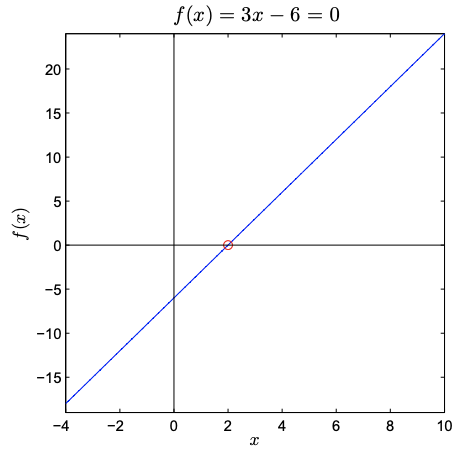
(a) linear function
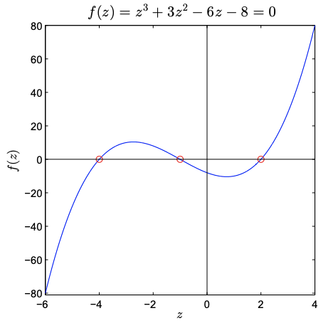
(b) nonlinear function
Figure 29.3: Solutions of univariate linear and nonlinear equations.
- Start with an initial guess or approximation for the root of a nonlinear system.
- Linearize the system around that initial approximation and solve the resulting linear system to find a better approximation for the root.
- Continue linearizing and solving until satisfied with the accuracy of the approximation.
This approach is identical for both univariate (one equation in one variable) and multivariate ( \(n\) equations in \(n\) variables) systems. We will first consider the univariate case and then extend our analysis to the multivariate case.