
29.2: Univariate Newton
- Page ID
- 55713

Method
Given a univariate function \(f(z)\), we wish to find a real zero/root \(Z\) of \(f\) such that \(f(Z)=0\). Note that \(z\) is any real value (for which the function is defined), whereas \(Z\) is a particular value of \(z\) at which \(f(z=Z)\) is zero; in other words, \(Z\) is a root of \(f(z)\).
We first start with an initial approximation (guess) \(\hat{z}^{0}\) for the zero \(Z\). We next approximate the function \(f(z)\) with its first-order Taylor series expansion around \(\hat{z}^{0}\), which is the line tangent to \(f(z)\) at \(z=\hat{z}^{0}\) \[f_{\text {linear }}^{0}(z) \equiv f^{\prime}\left(\hat{z}^{0}\right)\left(z-\hat{z}^{0}\right)+f\left(\hat{z}^{0}\right) .\] We find the zero \(\hat{z}^{1}\) of the linearized system \(f_{\text {linear }}^{0}(z)\) by \[f_{\text {linear }}^{0}\left(\hat{z}^{1}\right) \equiv f^{\prime}\left(\hat{z}^{0}\right)\left(\hat{z}^{1}-\hat{z}^{0}\right)+f\left(\hat{z}^{0}\right)=0,\] which yields \[\hat{z}^{1}=\hat{z}^{0}-\frac{f\left(\hat{z}^{0}\right)}{f^{\prime}\left(\hat{z}^{0}\right)} .\] We then repeat the procedure with \(\hat{z}^{1}\) to find \(\hat{z}^{2}\) and so on, finding successively better approximations to the zero of the original system \(f(z)\) from our linear approximations \(f_{\text {linear }}^{k}(z)\) until we reach \(\hat{z}^{N}\) such that \(\left|f\left(\hat{z}^{N}\right)\right|\) is within some desired tolerance of zero. (To be more rigorous, we must relate \(\left|f\left(\hat{z}^{N}\right)\right|\) to \(\left|Z-\hat{z}^{N}\right|\).)
Example
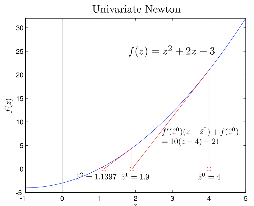
The first few steps of the following example have been illustrated in Figure 29.4.
We wish to use the Newton method to find a solution to the equation \[z^{2}+2 z=3 .\] We begin by converting the problem to a root-finding problem \[f(Z)=Z^{2}+2 Z-3=0 .\] We next note that the derivative of \(f\) is given by \[f^{\prime}(z)=2 z+2 .\] We start with initial guess \(\hat{z}^{0}=4\). We then linearize around \(\hat{z}^{0}\) to get \[f_{\text {linear }}^{0}(z) \equiv f^{\prime}\left(\hat{z}^{0}\right)\left(z-\hat{z}^{0}\right)+f\left(\hat{z}^{0}\right)=10(z-4)+21 .\] We solve the linearized system \[f_{\text {linear }}^{0}\left(\hat{z}^{1}\right) \equiv 10(z-4)+21=0\] to find the next approximation for the root of \(f(z)\), \[\hat{z}^{1}=1.9 .\] We repeat the procedure to find \[\begin{aligned} f_{\text {linear }}^{1}(z) \equiv f^{\prime}\left(\hat{z}^{1}\right)\left(z-\hat{z}^{1}\right)+f\left(\hat{z}^{1}\right) &=5.8(z-1.9)+4.41 \\ f_{\text {linear }}^{1}\left(\hat{z}^{2}\right) &=0 \\ \hat{z}^{2} &=1.1397 ; \\ f_{\text {linear }}^{2}(z) \equiv f^{\prime}\left(\hat{z}^{2}\right)\left(z-\hat{z}^{2}\right)+f\left(\hat{z}^{2}\right) &=4.2793(z-1.1397)+0.5781 \\ f_{\text {linear }}^{2}\left(\hat{z}^{3}\right) &=0 \\ \hat{z}^{3} &=1.0046 \end{aligned}\] Note the rapid convergence to the actual root \(Z=1\). Within three iterations the error has been reduced to \(0.15 \%\) of its original value.
Algorithm
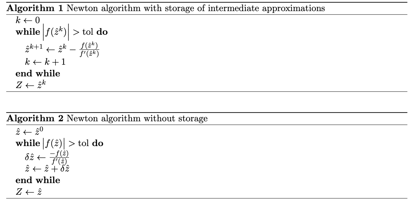
The algorithm for the univariate Newton’s method is a simple while loop. If we wish to store the intermediate approximations for the zero, the algorithm is shown in Algorithm \(\underline{1}\). If we don’t need to save the intermediate approximations, the algorithm is shown in Algorithm \(\underline{2}\).
If, for some reason, we cannot compute the derivative \(f^{\prime}\left(\hat{z}^{k}\right)\) directly, we can substitute the finite difference approximation of the derivative (see Chapter 3 ) for some arbitrary (small) given \(\Delta z\), which, for the backward difference is given by \[f^{\prime}\left(\hat{z}^{k}\right) \approx \frac{f\left(\hat{z}^{k}\right)-f\left(\hat{z}^{k}-\Delta z\right)}{\Delta z} .\] In practice, for \(\Delta z\) sufficiently small (but not too small - round-off), Newton with approximate derivative will behave similarly to Newton with exact derivative.
There also exists a method, based on Newton iteration, that directly incorporates a finite difference approximation of the derivative by using the function values at the two previous iterations (thus requiring two initial guesses) to construct \[f^{\prime}\left(\hat{z}^{k}\right) \approx \frac{f\left(\hat{z}^{k}\right)-f\left(\hat{z}^{k-1}\right)}{\hat{z}^{k}-\hat{z}^{k-1}} .\] This is called the secant method because the linear approximation of the function is no longer a line tangent to the function, but a secant line. This method works well with one variable (with a modest reduction in convergence rate); the generalization of the secant method to the multivariate case (and quasi-Newton methods) is more advanced.
Another root-finding method that works well (although slowly) in the univariate case is the bisection (or "binary chop") method. The bisection method finds the root within a given interval by dividing the interval in half on each iteration and keeping only the half whose function evaluations at its endpoints are of opposite sign - and which, therefore, must contain the root. This method is very simple and robust - it works even for non-smooth functions - but, because it fails to exploit any information regarding the derivative of the function, it is slow. It also cannot be generalized to the multivariate case.
Convergence Rate
When Newton works, it works extremely fast. More precisely, if we denote the error in Newton’s approximation for the root at the \(k^{\text {th }}\) iteration as \[\epsilon^{k}=\hat{z}^{k}-Z,\] then if
(\(i\)) \(f(z)\) is smooth (e.g., the second derivative exists),
(\(ii\)) \(f^{\prime}(Z) \neq 0\) (i.e., the derivative at the root is nonzero), and
(\(iii\)) \(\left|\epsilon^{0}\right|\) (the error of our initial guess) is sufficiently small,
we can show that we achieve quadratic (i.e., \(\left.\epsilon^{k+1} \sim\left(\epsilon^{k}\right)^{2}\right)\) convergence: \[\epsilon^{k+1} \sim\left(\epsilon^{k}\right)^{2}\left(\frac{1}{2} \frac{f^{\prime \prime}(Z)}{f^{\prime}(Z)}\right) .\] Each iteration doubles the number of correct digits; this is extremely fast convergence. For our previous example, the sequence of approximations obtained is shown in Table 29.1. Note that the doubling of correct digits applies only once we have at least one correct digit. For the secant method, the convergence rate is slightly slower: \[\epsilon^{k+1} \sim\left(\epsilon^{k}\right)^{\gamma},\] where \(\gamma \approx 1.618\).
Proof. A sketch of the proof for Newton’s convergence rate is shown below:
| iteration | approximation | number of correct digits |
|---|---|---|
| 0 | 4 | 0 |
| 1 | \(1.9\) | 1 |
| 2 | \(1.1 \ldots\) | 1 |
| 3 | \(1.004 \ldots\) | 3 |
| 4 | \(1.000005 \ldots\) | 6 |
| 5 | \(1.00000000006 \ldots\) | 12 |
Table 29.1: Convergence of Newton for the example problem. \[\begin{aligned} \hat{z}^{k+1} &=\hat{z}^{k}-\frac{f\left(\hat{z}^{k}\right)}{f^{\prime}\left(\hat{z}^{k}\right)} \\ Z+\epsilon^{k+1} &=Z+\epsilon^{k}-\frac{f\left(Z+\epsilon^{k}\right)}{f^{\prime}\left(Z+\epsilon^{k}\right)} \\ \epsilon^{k+1} &=\epsilon^{k}-\frac{f(Z)+\epsilon^{k} f^{\prime}(Z)+\frac{1}{2}\left(\epsilon^{k}\right)^{2} f^{\prime \prime}(Z)+\cdots}{f^{\prime}(Z)+\epsilon^{k} f^{\prime \prime}(Z)+\cdots} \\ \epsilon^{k+1} &=\epsilon^{k}-\epsilon^{k} \frac{f^{\prime}(Z)+\frac{1}{2} \epsilon^{k} f^{\prime \prime}(Z)+\cdots}{f^{\prime}(Z)\left(1+\epsilon^{k} \frac{f^{\prime \prime}(Z)}{f^{\prime}(Z)}+\cdots\right)} \\ \epsilon^{k+1} &=\epsilon^{k}-\epsilon^{k} \frac{f^{\prime}(Z)\left(1+\frac{1}{2} \epsilon^{k} \frac{f^{\prime \prime}(Z)}{f^{\prime}(Z)}+\cdots\right.}{f^{\prime}(Z)\left(1+\epsilon^{k} \frac{f^{\prime \prime}(Z)}{f^{\prime}(Z)}+\cdots\right)} \end{aligned}\] since \(\frac{1}{1+\rho} \sim 1-\rho+\cdots\) for small \(\rho\), \[\begin{aligned} \epsilon^{k+1} &=\epsilon^{k}-\epsilon^{k}\left(1+\frac{1}{2} \epsilon^{k} \frac{f^{\prime \prime}(Z}{f^{\prime}(Z)}\right)\left(1-\epsilon^{k} \frac{f^{\prime \prime}(Z)}{f^{\prime}(Z)}\right)+\cdots \\ \epsilon^{k+1} &=\ell^{k}-\ell^{k}+\frac{1}{2}\left(\epsilon^{k}\right)^{2} \frac{f^{\prime \prime}(Z)}{f^{\prime}(Z)}+\cdots \\ \epsilon^{k+1} &=\frac{1}{2} \frac{f^{\prime \prime}(Z)}{f^{\prime}(Z)}\left(\epsilon^{k}\right)^{2}+\cdots \end{aligned}\] We thus confirm the quadratic convergence.
Note that, if \(f^{\prime}(Z)=0\), we must stop at equation \(\left(\underline{29.26)}\right.\) to obtain the linear (i.e., \(\epsilon^{k+1} \sim \epsilon^{k}\) ) convergence rate \[\begin{aligned} \epsilon^{k+1} &=\epsilon^{k}-\frac{\frac{1}{2}\left(\epsilon^{k}\right)^{2} f^{\prime \prime}(Z)+\cdots}{\epsilon^{k} f^{\prime \prime}(Z)} \\ \epsilon^{k+1} &=\frac{1}{2} \epsilon^{k}+\cdots . \end{aligned}\] In this case, we gain only a constant number of correct digits after each iteration. The bisection method also displays linear convergence.
Newton Pathologies
Although Newton often does work well and very fast, we must always be careful not to excite pathological (i.e., atypically bad) behavior through our choice of initial guess or through the nonlinear function itself.
For example, we can easily - and, thus, this might be less pathology than generally bad behavior - arrive at an "incorrect" solution with Newton if our initial guess is poor. For instance, in our earlier example of Figure 29.4, say that we are interested in finding a positive root, \(Z>0\), of \(f(z)\). If we had chosen an initial guess of \(\hat{z}^{0}=-4\) instead of \(\hat{z}^{0}=+4\), we would have (deservingly) found the root \(Z=-3\) instead of \(Z=1\). Although in the univariate case we can often avoid this behavior by basing our initial guess on a prior inspection of the function, this approach becomes more difficult in higher dimensions.
Even more diabolical behavior is possible. If the nonlinear function has a local maximum or minimum, it is often possible to excite oscillatory behavior in Newton through our choice of initial guess. For example, if the linear approximations at two points on the function both return the other point as their solution, Newton will oscillate between the two indefinitely and never converge to any roots. Similarly, if the first derivative is not well behaved in the vicinity of the root, then Newton may diverge to infinity.
We will later address these issues (when possible) by continuation and homotopy methods.