2.1: Trusses
- Page ID
- 44531
\( \newcommand{\vecs}[1]{\overset { \scriptstyle \rightharpoonup} {\mathbf{#1}} } \)
\( \newcommand{\vecd}[1]{\overset{-\!-\!\rightharpoonup}{\vphantom{a}\smash {#1}}} \)
\( \newcommand{\dsum}{\displaystyle\sum\limits} \)
\( \newcommand{\dint}{\displaystyle\int\limits} \)
\( \newcommand{\dlim}{\displaystyle\lim\limits} \)
\( \newcommand{\id}{\mathrm{id}}\) \( \newcommand{\Span}{\mathrm{span}}\)
( \newcommand{\kernel}{\mathrm{null}\,}\) \( \newcommand{\range}{\mathrm{range}\,}\)
\( \newcommand{\RealPart}{\mathrm{Re}}\) \( \newcommand{\ImaginaryPart}{\mathrm{Im}}\)
\( \newcommand{\Argument}{\mathrm{Arg}}\) \( \newcommand{\norm}[1]{\| #1 \|}\)
\( \newcommand{\inner}[2]{\langle #1, #2 \rangle}\)
\( \newcommand{\Span}{\mathrm{span}}\)
\( \newcommand{\id}{\mathrm{id}}\)
\( \newcommand{\Span}{\mathrm{span}}\)
\( \newcommand{\kernel}{\mathrm{null}\,}\)
\( \newcommand{\range}{\mathrm{range}\,}\)
\( \newcommand{\RealPart}{\mathrm{Re}}\)
\( \newcommand{\ImaginaryPart}{\mathrm{Im}}\)
\( \newcommand{\Argument}{\mathrm{Arg}}\)
\( \newcommand{\norm}[1]{\| #1 \|}\)
\( \newcommand{\inner}[2]{\langle #1, #2 \rangle}\)
\( \newcommand{\Span}{\mathrm{span}}\) \( \newcommand{\AA}{\unicode[.8,0]{x212B}}\)
\( \newcommand{\vectorA}[1]{\vec{#1}} % arrow\)
\( \newcommand{\vectorAt}[1]{\vec{\text{#1}}} % arrow\)
\( \newcommand{\vectorB}[1]{\overset { \scriptstyle \rightharpoonup} {\mathbf{#1}} } \)
\( \newcommand{\vectorC}[1]{\textbf{#1}} \)
\( \newcommand{\vectorD}[1]{\overrightarrow{#1}} \)
\( \newcommand{\vectorDt}[1]{\overrightarrow{\text{#1}}} \)
\( \newcommand{\vectE}[1]{\overset{-\!-\!\rightharpoonup}{\vphantom{a}\smash{\mathbf {#1}}}} \)
\( \newcommand{\vecs}[1]{\overset { \scriptstyle \rightharpoonup} {\mathbf{#1}} } \)
\(\newcommand{\longvect}{\overrightarrow}\)
\( \newcommand{\vecd}[1]{\overset{-\!-\!\rightharpoonup}{\vphantom{a}\smash {#1}}} \)
\(\newcommand{\avec}{\mathbf a}\) \(\newcommand{\bvec}{\mathbf b}\) \(\newcommand{\cvec}{\mathbf c}\) \(\newcommand{\dvec}{\mathbf d}\) \(\newcommand{\dtil}{\widetilde{\mathbf d}}\) \(\newcommand{\evec}{\mathbf e}\) \(\newcommand{\fvec}{\mathbf f}\) \(\newcommand{\nvec}{\mathbf n}\) \(\newcommand{\pvec}{\mathbf p}\) \(\newcommand{\qvec}{\mathbf q}\) \(\newcommand{\svec}{\mathbf s}\) \(\newcommand{\tvec}{\mathbf t}\) \(\newcommand{\uvec}{\mathbf u}\) \(\newcommand{\vvec}{\mathbf v}\) \(\newcommand{\wvec}{\mathbf w}\) \(\newcommand{\xvec}{\mathbf x}\) \(\newcommand{\yvec}{\mathbf y}\) \(\newcommand{\zvec}{\mathbf z}\) \(\newcommand{\rvec}{\mathbf r}\) \(\newcommand{\mvec}{\mathbf m}\) \(\newcommand{\zerovec}{\mathbf 0}\) \(\newcommand{\onevec}{\mathbf 1}\) \(\newcommand{\real}{\mathbb R}\) \(\newcommand{\twovec}[2]{\left[\begin{array}{r}#1 \\ #2 \end{array}\right]}\) \(\newcommand{\ctwovec}[2]{\left[\begin{array}{c}#1 \\ #2 \end{array}\right]}\) \(\newcommand{\threevec}[3]{\left[\begin{array}{r}#1 \\ #2 \\ #3 \end{array}\right]}\) \(\newcommand{\cthreevec}[3]{\left[\begin{array}{c}#1 \\ #2 \\ #3 \end{array}\right]}\) \(\newcommand{\fourvec}[4]{\left[\begin{array}{r}#1 \\ #2 \\ #3 \\ #4 \end{array}\right]}\) \(\newcommand{\cfourvec}[4]{\left[\begin{array}{c}#1 \\ #2 \\ #3 \\ #4 \end{array}\right]}\) \(\newcommand{\fivevec}[5]{\left[\begin{array}{r}#1 \\ #2 \\ #3 \\ #4 \\ #5 \\ \end{array}\right]}\) \(\newcommand{\cfivevec}[5]{\left[\begin{array}{c}#1 \\ #2 \\ #3 \\ #4 \\ #5 \\ \end{array}\right]}\) \(\newcommand{\mattwo}[4]{\left[\begin{array}{rr}#1 \amp #2 \\ #3 \amp #4 \\ \end{array}\right]}\) \(\newcommand{\laspan}[1]{\text{Span}\{#1\}}\) \(\newcommand{\bcal}{\cal B}\) \(\newcommand{\ccal}{\cal C}\) \(\newcommand{\scal}{\cal S}\) \(\newcommand{\wcal}{\cal W}\) \(\newcommand{\ecal}{\cal E}\) \(\newcommand{\coords}[2]{\left\{#1\right\}_{#2}}\) \(\newcommand{\gray}[1]{\color{gray}{#1}}\) \(\newcommand{\lgray}[1]{\color{lightgray}{#1}}\) \(\newcommand{\rank}{\operatorname{rank}}\) \(\newcommand{\row}{\text{Row}}\) \(\newcommand{\col}{\text{Col}}\) \(\renewcommand{\row}{\text{Row}}\) \(\newcommand{\nul}{\text{Nul}}\) \(\newcommand{\var}{\text{Var}}\) \(\newcommand{\corr}{\text{corr}}\) \(\newcommand{\len}[1]{\left|#1\right|}\) \(\newcommand{\bbar}{\overline{\bvec}}\) \(\newcommand{\bhat}{\widehat{\bvec}}\) \(\newcommand{\bperp}{\bvec^\perp}\) \(\newcommand{\xhat}{\widehat{\xvec}}\) \(\newcommand{\vhat}{\widehat{\vvec}}\) \(\newcommand{\uhat}{\widehat{\uvec}}\) \(\newcommand{\what}{\widehat{\wvec}}\) \(\newcommand{\Sighat}{\widehat{\Sigma}}\) \(\newcommand{\lt}{<}\) \(\newcommand{\gt}{>}\) \(\newcommand{\amp}{&}\) \(\definecolor{fillinmathshade}{gray}{0.9}\)Introduction
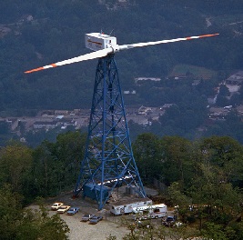
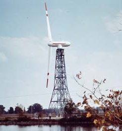
A truss is an assemblage of long, slender structural elements that are connected at their ends. Trusses find substantial use in modern construction, for instance as towers (see Figure 1), bridges, scaffolding, etc. In addition to their practical importance as useful structures, truss elements have a dimensional simplicity that will help us extend further the concepts of mechanics introduced in the modules dealing with uniaxial response. This module will also use trusses to introduce important concepts in statics and numerical analysis that will be extended in later modules to more general problems.
Trusses are often used to stiffen structures, and most people are familiar with the often very elaborate systems of cross-bracing used in bridges. The truss bracing used to stiffen the towers of suspension bridges against buckling are hard to miss, but not everyone notices the vertical truss panels on most such bridges that serve to stiffen the deck against flexural and torsional deformation.
Many readers will have seen the very famous movie, taken on November 7, 1940, by Barney Elliott of The Camera Shop in Tacoma, Washington. The wind was gusting up to 42 mph that day, and induced a sequence of spectacular undulations and eventual collapse of the Tacoma Narrows bridge (An interactive instructional videodisk of the Tacoma Narrows Bridge collapse is available from Wiley Educational Software (ISBN 0-471-87320-9).). This bridge was built using relatively short I-beams for deck stiffening rather than truss panels, reportedly for aesthetic reasons; bridge designs of the period favored increasingly slender and graceful-appearing structures. Even during construction, the bridge became well known for its alarming tendency to sway in the wind, earning it the local nickname "Galloping Gertie."
Truss stiffeners were used when the bridge was rebuilt in 1950, and the new bridge was free of the oscillations that led to the collapse of its predecessor. This is a good example of one important use of trusses, but it is probably an even better example of the value of caution and humility in engineering. The glib answers often given for the original collapse — resonant wind gusts, von Karman vortices, etc. — are not really satisfactory beyond the obvious statement that the deck was not stiff enough. Even today, knowledgeable engineers argue about the very complicated structural dynamics involved. Ultimately, many uncertainties exist even in designs completed using very modern and elaborate techniques. A wise designer will never fully trust a theoretical result, computer-generated or not, and will take as much advantage of experience and intuition as possible.
Statics analysis of forces
Newton observed that a mass accelerates according to the vector sum of forces applied to it: \(\sum F = ma\). (Vector quantities indicated by boldface type.) In structures that are anchored so as to prevent motion, there is obviously no acceleration and the forces must sum to zero. This vector equation has as many scalar components as the dimensionality of the problem; for two-dimensional cases we have:
\[\sum F_x = 0 \nonumber \]
\[\sum F_y = 0 \nonumber \]
where \(F_x\) and \(F_y\) are the components of \(F\) in the \(x\) and \(y\) cartesian coordinate directions. These two equations, which we can interpret as constraining the structure against translational motion in the \(x\) and \(y\) directions, allow us to solve for at most two unknown forces in structural problems. If the structure is constrained against rotation as well as translation, we can add a moment equation that states that the sum of moments or torques in the \(x-y\) plane must also add to zero:
\[\sum M_{xy} = 0 \nonumber \]
In two dimensions, then, we have three equations of static equilibrium that can be used to solve for unknown forces. In three dimensions, a third force equation and two more moment equations are added, for a total of six:
\[\begin{array} {c} {\sum F_x = 0 \ \ \ \ \ \ \sum M_{xy} = 0} \\ {\sum F_y = 0 \ \ \ \ \ \ \sum M_{xz} = 0} \\ {\sum F_z = 0 \ \ \ \ \ \ \sum M_{yz} = 0} \end{array} \nonumber \]
These equations can be applied to the structure as a whole, or we can (conceptually) remove a piece of the structure and consider the forces acting on the removed piece. A sketch of the piece, showing all forces acting on it, is called a free body diagram. If the number of unknown forces in the diagram is equal to or less than the number of available static equilibrium equations, the unknowns can be solved in a straightforward manner; such problems are termed statically determinate. Note that these equilibrium equations do not assume anything about the material from which the structure is made, so the resulting forces are also independent of the material.
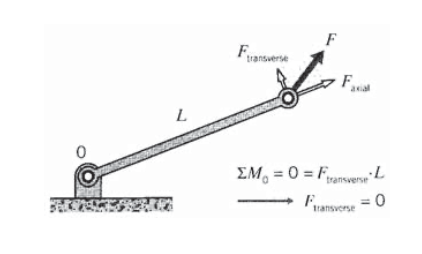
In the analyses to be considered here, the truss elements are assumed to be joined together by pins or other such connections that allow free rotation around the joint. As seen in the free-body diagram of Figure 2, this inability to resist rotation implies that the force acting on a truss element’s pin joint must be in the element’s axial direction: any transverse component would tend to cause rotation, and if the element is to be in static equilibrium the moment equation forces the transverse component to vanish. If the element ends were to be welded or bolted rather than simply pinned, the end connection could transmit transverse forces and bending moments into the element. Such a structure would then be called a frame rather than a truss, and its analysis would have to include bending effects. Such structures will be treated in the Module on Bending.
Knowing that the force in each truss element must be be in the element’s axial direction is the key to solving for the element forces in trusses that contain many elements. Each element meeting at a pin joint will pull or push on the pin depending on whether the element is in tension or compression, and since the pin must be in static equilibrium the sum of all element forces acting on the pin must equal the force that is externally applied to the pin:
\[\sum_{e} F_i^e = F_i \nonumber \]
Here the \(e\) superscript indicates the vector force supplied by the element on the \(i^{th}\) pin in the truss and \(F_i\) in the force externally applied to that pin. The summation is over all the elements connected to the pin.
The very simple two-element truss often found in high school physics books and shown in Figure 3 can be analyzed this way. Intuition tells us that the upper element, connecting joints \(A\) and \(B\), is in tension while element \(BC\) is in compression. In more complicated problems it is not always possible to determine the sign of the element force by inspection, but it doesn’t matter. In sketching the free body diagrams for the pins, the load can be drawn in either direction; if the guess turns out to be wrong, the solution will give a negative value for the force magnitude.
The unknown forces on the connecting pin \(B\) are in the direction of the elements attached to it, and since there are only two such forces they may be determined from the two static equilibrium force equations:
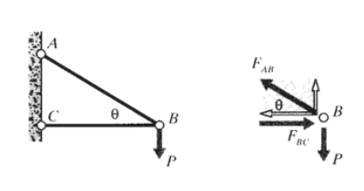
\[\sum F_y = 0 = + F_{AB} \sin \theta - P \Rightarrow F_{AB} = \dfrac{P}{\sin \theta}\nonumber \]
\[\sum F_x = 0 = -F_{AB} \cos \theta + F_{BC} \Rightarrow F_{BC} = F_{AB} \cos \theta = \dfrac{P}{\tan \theta}\nonumber \]
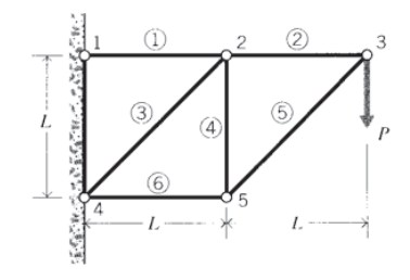
In more complicated trusses, the general approach is to start at a pin joint containing no more than two elements having unknown forces, and then work from joint to joint using the element forces from the previous step to reduce the number of unknowns. Consider the 6-element truss shown in Figure 4, in which the joints and elements are numbered as indicated, with the element numbers appearing in circles. Joint 3 is a natural starting point, since only forces \(F_2\) and \(F_5\) appear as unknowns. Once F5 is found, an analysis of joint 5 has only forces \(F_4\) and \(F_6\) as unknowns. Finally, the free-body diagram of node 2 can be completed, since only \(F_1\) and \(F_3\) are now unknown. The force analysis is then complete.
There are often many ways to complete problems such as this, perhaps with some being easier than others. Another approach might be to start at one of the joints at the wall; i.e. joint 1 or joint 4. The problem as originally stated gives these joints as having fixed displacements rather than specified forces. This is an example of a mixed boundary value problem, with some parts of the boundary having specified forces and the remaining parts having specified displacements. Such problems are generally more difficult, and require more mathematical information for their solution than problems having only one or the other type of boundary condition. However, in the statically determinate problems, the structure can be converted to a load-only type by invoking static equilibrium on the structure as a whole. The fixed-displacement boundary conditions are then replaced by reaction forces that are set up at the points of constraint.
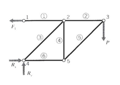
Moment equilibrium equations were not useful in the joint-by-joint analysis described earlier, since individual elements cannot support moments. But as seen in Figure 5, we can consider the 6-element truss as a whole and take moments around joint 4. With counterclockwise-tending moments being positive, this gives
\[\sum M_4 = 0 = F_1 \times L - P \times 2 L \Rightarrow F_1 = 2P\nonumber \]
The force \(F_1\) is the force applied by the wall to joint 1, and this is obviously equal to the tensile force in element 1. There can be no vertical component of this reaction force, since the element forces must be axial and only element 1 is connected to joint 1. At joint 4, reaction forces Rx and Ry can act in both the \(x\) and \(y\) directions since element 3 is not perpendicular to the wall. These reaction forces can be found by invoking horizontal and vertical equilibrium:
\[\sum F_x = 0 = -F_1 + R_x \Rightarrow R_x = F_1 = 2P\nonumber \]
\[\sum F_y = 0 = + R_y - P \Rightarrow R_y = P\nonumber \]
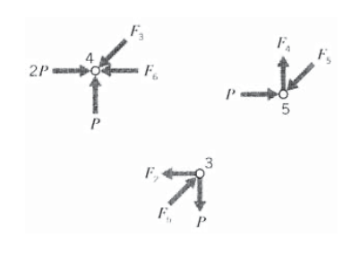
A joint-by-joint analysis can now be started from joint 4, since only two unknown forces act there (see Figure 6). For vertical equilibrium, \(F_3 \cos 45 = P\), so \(F_3 = \sqrt{2} P\). Then for horizontal equilibrium \(F_6 + F_3 \cos 45 = 2P\), so \(F_6 = P\). Now moving to joint 5, horizontal equilibrium gives \(F_5 \cos 45 = P\) so \(F_5 = F_3 = \sqrt{2} P\), and vertical equilibrium gives \(F_4 = F_5 \cos 45\) so \(F_4 = P\). Finally, at joint 3 horizontal equilibrium gives \(F_2 = F_5 \cos 45\) so \(F_2 = P\).
In actual truss design, once each element’s force is known its cross-sectional area can then be calculated so as to keep the element stress according to \(\sigma = P/A\) safely less than the material’s yield point. Elements in compression, however, must be analyzed for buckling as well, since their ratios of \(EI\) to \(L^2\) are generally low. The buckling load can be increased substantially by bracing the element against sideward deflection, and this bracing is evident in most bridges and cranes. Also, the truss elements are usually held together by welded or bolted joints rather than pins. These joints can carry some bending moments, which helps stiffen the truss against buckling.
Deflections
It may be important in some applications that the truss be stiff enough to keep the deformations inside specified limits. Astronomical telescopes are an example, since deflection of the structure supporting the optical assemblies can degrade the focusing ability of the instrument. A typical derrick or bridge, however, is probably more likely to be strength rather than stiffness-critical, so it might appear deflections would be relatively unimportant. However, it will be seen that consideration of deflections is necessary to solve the great number of structures that are not statically determinate. The following sections treat truss deflections for both these reasons.
Geometrical approach
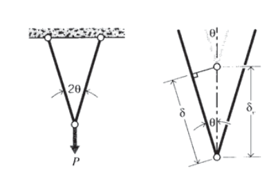
Once the axial force in each truss element is known, the individual element deformations follow directly using \(\delta = PL/AE\). The deflection of any point in the truss can then be determined geometrically, invoking the requirement that the elements remain pinned together at their attachment points. In the symmetric two-element truss shown in Figure 7, joint \(B\) will obviously deflect downward vertically. The relation between the the axial deformation \(\delta\) of the elements and the vertical deflection of the joint \(\delta_v\) is then seen to be
\[\delta_v = \dfrac{\delta}{\cos \theta}\nonumber \]
It is assumed here that the deformation is small enough that the gross aspects of the geometry are essentially unchanged; in this case, that the angle \(\theta\) is the same before and after the load is applied.
In geometrical analyses of more complicated trusses, it is sometimes convenient to visualize unpinning the elements at a selected joint, letting the elements elongate or shrink according to the axial force they are transmitting, and then swinging them around the still-pinned joint until the pin locations match up again. The motion of the unpinned ends would trace out circular paths, but if the deflections are small the path can be approximated as a straight line perpendicular to the element axis. The joint position can then be computed from Pythagorean relationships.
In the earlier two-element truss shown in Figure 3, we had \(P_{AB} = P/ \sin \theta\) and \(P_{BC} = P/ \tan \theta\). If the pin at joint \(B\) were removed, the element deflections would be
\[\delta_{AB} = \dfrac{P}{\sin \theta} \left ( \dfrac{L}{AE} \right )_{AB} \text{ (tension)}\nonumber \]
\[\delta_{BC} = \dfrac{P}{\tan \theta} \left ( \dfrac{L}{AE} \right )_{BC} \text{ (compression)}\nonumber \]
The total downward deflection of joint \(B\) is then
\[\delta_v = \delta_1 + \delta_2= \dfrac{\delta_{AB}}{\sin \theta} + \dfrac{\delta_{BC}}{\tan \theta}\nonumber \]
\[= \dfrac{P}{\sin^2 \theta} \left ( \dfrac{L}{AE} \right )_{AB} + \dfrac{P}{\tan^2 \theta} \left ( \dfrac{L}{AE} \right )_{BC} \nonumber \]
These deflections are shown in Figure 8.
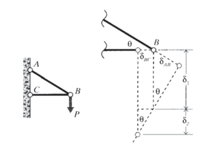
The horizontal deflection \(\delta_h\) of the pin is easier to compute, since it is just the contraction of element \(BC\):
\[\delta_h = \delta_{BC} = \dfrac{P}{\tan \theta} \left ( \dfrac{L}{AE} \right )_{BC} \nonumber \]
Energy approach
The geometrical approach to truss deformation analysis can be rather tedious, especially as problems become larger. Many problems can be solved more easily using a strain energy rather than force-at-a-point approach. The total strain energy \(U\) in a single elastically loaded truss element is
\[U = \int P\ d\delta\nonumber \]
The increment of deformation \(d\delta\) is related to a corresponding increment of load \(dP\) by
\[\delta = \dfrac{PL}{AE} \Rightarrow d\delta = \dfrac{L}{AE} dP\nonumber \]
The strain energy is then
\[U = \int P \dfrac{L}{AE} dP = \dfrac{P^2L}{2AE}\nonumber \]
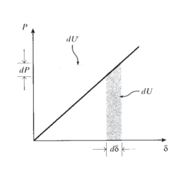
The incremental increase in strain energy corresponding to an increase in deformation \(d\delta\) is just \(dU = P d\delta\). If the force-elongation curve is linear, this is identical to the increase in the quantity called the complimentary strain energy: \(dU^c = \delta dP\). These quantities are depicted in Figure 9. Now consider a system with many joints, subjected to a number of loads acting at different joints. If we were to increase the \(i^{th}\) load slightly while holding all the other loads constant, the increase in the total complementary energy of the system would be
\[dU^c = \delta_i dP_i\nonumber \]
where \(\delta_i\) is the displacement that would occur at the location of \(P_i\), moving in the same direction as the force vector for \(P_i\). Rearranging,
\[\delta_i = \dfrac{\partial U^c}{\partial P_i}\nonumber \]
and since \(U^c = U\):
\[\delta_i = \dfrac{\partial U}{\partial P_i} \nonumber \]
Hence the displacement at a given point is the derivative of the total strain energy with respect to the load acting at that point. This provides the basis of an extremely useful method of displacement analysis known as Castigliano’s Theorem(From the 1873 thesis of the Italian engineer Alberto Castigliano (1847–1884), at the Turin Polytechnical Institute.), which can be stated for truss problems as the following recipe:
- Let the load applied at the joint whose deformation is sought, in the direction of the desired deformation, be written as an algebraic variable, say \(Q\). If the load is known numerically, replace the number with a letter. If there is no load at the desired location and direction, put an imaginary one there that will be set to zero at the end of the problem.
- Solve for the forces \(F_i(Q)\) in each truss element, each of which may be dependent on the load \(Q\) assigned in the previous step.
- Use these forces to compute the strain energy for each element, and sum the energies in each element to obtain the total strain energy for the truss:
\[U_{tot} = \sum_{i} U_i = \sum_i \dfrac{F_i^2 L_i}{2A_i E_i} \nonumber \]
Each term in this summation may contain the variable \(Q\). - The deformation congruent to \(Q\), i.e. the deformation at the point where \(Q\) is applied and in the same direction as \(Q\), is then
\[\delta_Q = \dfrac{\partial U_{tot}}{\partial Q} = \sum_i \dfrac{F_i L_i}{A_i E_i} \dfrac{\partial F_i (Q)}{\partial Q} \nonumber \] - The load \(Q\) is replaced by its numerical value, if known. Or by zero, if it was an imaginary load in the first place.
Applying this method to the vertical deflection of the two-element truss of Figure 3, the problem already has a force in the required direction, the applied downward load \(P\). The forces have already been shown to be \(P_{AB} = P/ \sin \theta\) and \(P_{BC} = P/ \tan \theta\), so the vertical deflection can be written immediately as
\[\begin{align*} \delta_v &= P_{AB} \left ( \dfrac{L}{AE} \right )_{AB} \dfrac{\partial P_{AB}}{\partial P} + P_{BC} \left ( \dfrac{L}{AE} \right )_{BC} \dfrac{\partial P_{BC}}{\partial P} \\[4pt] &=\dfrac{P}{\sin \theta} \left ( \dfrac{L}{AE} \right )_{AB} \dfrac{1}{\sin \theta} + \dfrac{P}{\tan \theta} \left ( \dfrac{L}{AE} \right )_{AB} \dfrac{1}{\sin \theta} + \dfrac{P}{\tan \theta} \left ( \dfrac{AE}{L} \right )_{BC} \dfrac{1}{\tan \theta} \end{align*} \]
This is identical to the expression obtained from geometric considerations. The energy method didn’t save too many algebraic steps in this case, but it avoided having to visualize and idealize the displacements geometrically.
If the horizontal displacement at joint \(B\) is desired, the method requires that a horizontal force exist at that point. One isn’t given, so we place an imaginary one there, say \(Q\). The truss is then reanalyzed statically to find how the element forces are influenced by this new force \(Q\). The upper element force is \(P_{AB} = P/\sin \theta\) as before, and the lower element force becomes \(P_{BC} = P/ \tan \theta - Q\). Repeating the Castigliano process, but now differentiating with respect to \(Q\)
\[\delta_h = P_{AB} \left ( \dfrac{L}{AE} \right )_{AB} \dfrac{\partial P_{AB}}{\partial P} + P_{BC} \left ( \dfrac{L}{AE} \right )_{BC} \dfrac{\partial P_{BC}}{\partial P}\nonumber \]
\[= \dfrac{P}{\sin \theta} \left ( \dfrac{L}{AE} \right )_{AB} \cdot 0 + \left (\dfrac{P}{\tan \theta} - Q \right ) \left ( \dfrac{L}{AE} \right )_{BC} (-1)\nonumber \]
The first term vanishes upon differentiation since \(Q\) did not appear in the expression for \(P_{AB}\). This is the method’s way of noticing that the horizontal deflection is determined completely by the contraction of element \(BC\). Upon setting \(Q = O\), the final result is
\[\delta_h = -\dfrac{P}{\tan \theta} \left ( \dfrac{AE}{L} \right )_{BC}\nonumber \]
as before.
Consider the 6-element truss of Figure 4 whose individual element forces were found earlier by free body diagrams. We are seeking the vertical deflection of node 3, which is congruent to the force \(P\). Using Castigliano’s method, this deflection is the derivative of the total strain energy with respect to \(P\). Equivalently, we can differentiate the strain energy of each element with respect to \(P\) individually, and then add the contributions of each element to obtain the final result:
\[\delta_P = \dfrac{\partial}{\partial P} \sum_i \dfrac{F_i^2L_i}{2A_i E_i} = \sum_i \left (\dfrac{F_i L_i}{A_i E_i} \dfrac{\partial F_i}{\partial P} \right )\nonumber \]
To systemize this approach, we can form a table of needed parameters as follows:
| \(i\) | \(F_i\) | \(\dfrac{L_i}{A_iE_i}\) | \(\dfrac{\partial F_i}{\partial P\) | \(\dfrac{F_i L_i}{A_i E_i} \dfrac{\partial F_i}{\partial P}\) |
| 1 | \(2P\) | \(L/AE\) | 2 | \(4PL/AE\) |
| 2 | \(P\) | \(L/AE\) | 1 | \(PL/AE\) |
| 3 | \(\sqrt{2} P\) | \(\sqrt{2} L/AE\) | \(\sqrt{2}\) | \(2.83 PL/AE\) |
| 4 | \(P\) | \(L/AE\) | 1 | \(PL/AE\) |
| 5 | \(\sqrt{2} P\) | \(\sqrt{2} L/AE\) | \(\sqrt{2}\) | \(2.83 PL/AE\) |
| 6 | \(P\) | \(L/AE\) | 1 | \(PL/AE\) |
If for instance we have as numerical parameters \(P = 1000\ lbs\), \(L = 100\ in\), \(E = 30\ Mpsi\) and \(A = 0.5\ in^2\), then \(\delta_P = 0.0844\ in\).
Statically indeterminate trusses
It has already been noted that that the element forces in the truss problems treated up to now do not depend on the properties of the materials used in their construction, just as the stress in a simple tension test is independent of the material. This result, which certainly makes the problem easier to solve, is a consequence of the earlier problems being statically determinate; i.e. able to be solved using only the equations of static equilibrium. Statical determinacy, then, is an important aspect of the difficulty we can expect in solving the problem. Not all problems are statically determinate, and one consequence of this indeterminacy is that the forces in the structure may depend on the material properties.
After performing a static analysis of the truss as a whole to find reaction forces at the supports, we typically try to find the element forces using the joint-at-a-time method described above. However, there can be at most two unknown forces at a pin joint in a two-dimensional truss problem if the joint is to be solved using statics alone, since the moment equation does not provide usable information in this case. If more unknowns are present no matter in which order the truss joints are analyzed, then a number of additional equations equal to the remaining unknowns must be found. These extra equations are those enforcing compatibility of the various joint displacements, each of which must be such as to keep the truss joints pinned together.
A simple example, just two truss elements acting in parallel as shown in Figure 10, will show the approach needed. Here the compatibility condition is just
\[\delta_A = \delta_B\nonumber \]
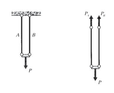
The individual element displacements are related to the element forces by \(\delta = PL/AE\), which is material- dependent and can be termed a constitutive equation because it reflects the material’s mechanical constitution. Combining this with the compatibility condition gives
\[\dfrac{P_AL}{A_A E_A} = \dfrac{P_BL}{A_BE_B} \Rightarrow P_B = P_A \dfrac{A_BE_B}{A_AE_A}\nonumber \]
Finally, the individual element forces must add up to the total applied load \(P\) in order to satisfy equilibrium:
\[P = P_A + P_B = P_A + P_A \dfrac{A_BE_B}{A_A E_A} \Rightarrow P_A = P \left (\dfrac{1}{1 + (\tfrac{A_BE_B}{A_AE_A})} \right )\nonumber \]
Note that the final answer in the above example depends on the element dimensions and material stiffnesses, as promised. Here the geometrical compatibility condition was very simple and obvious, namely that the displacements of the two element end joints were identical. In more complex trusses these relations can be subtle, but tend to become more evident with practice.
Three different types of relations were used in the above problem: a compatibility equation, stating how the structure must deform kinematically in order to remain connected; a constitutive equation, embodying the stress-strain response of the material; and an equilibrium equation, stating that the forces must sum to zero if acceleration is to be avoided. These three concepts, made somewhat more general mathematically to handle geometrically more elaborate problems, underlie all of solid mechanics.
In the Module on Elastic Response, we noted that the stress in a tensile specimen is determined only by considerations of static equilibrium, being given by \(\sigma = P/A\) independent of the material properties. We see now that the statical determinacy depends, among other things, on the material being homogeneous, i.e. identical throughout. If the tensile specimen is composed of two subunits each having different properties, the stresses will be allocated differently among the two units, and the stresses will not be uniform. Whenever a stress or deformation formula is copied out of a handbook, the user must be careful to note the limitations of the underlying theory. The handbook formulae are usually applicable only to homogeneous materials in their linear elastic range, and higher-order theories must be used when these conditions are not met.
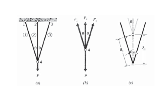
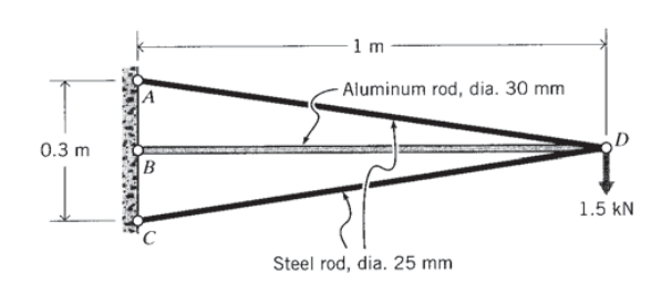
Figure 11(a) shows another statically indeterminate truss, with three elements having the same area and 11 modulus, but different lengths, meeting at a common node. At a glance, we can see node 4 has three elements meeting there whose forces are unknown, and this is one more than the useful equations of static equilibrium will be able to handle. This is also evident in the free-body diagram of Figure 11(b): horizontal and vertical equilibrium gives
\[\sum F_x = 0 = -F_1 + F_2 \to F_1 = F_2\nonumber \]
\[\sum F_y = 0 = -P + F_2 + F_1 \cos \theta + F_3 \cos \theta \to F_2 + 2 F_3 \cos \theta = P \nonumber \]
These two equations are clearly not sufficient to determine the unknowns \(F_1, F_2, F_3\). We need another equation, and it’s provided by requiring the deformation be such as to keep the truss pinned together at node 4. Since the symmetry of the problems tells us that the deflection there is straight downward, the diagram in Figure 11(c) can be used. And since the deflection is small relative to the lengths of the elements, the angle of element 3 remains essentially unchanged after deformation. This lets us write
\[\delta_3 = \delta_2 \cos \theta\nonumber \]
or
\[\dfrac{F_3L_3}{A_3E_3} = \dfrac{F_2L_2}{A_2E_2} \cos \theta \nonumber \]
Using \(A_2 = A_3\), \(E_2 = E_3\), \(L_3 = L\), and \(L_2 = L \cos \theta\), this becomes
\[F_3 = F_2 \cos^2 \theta\nonumber \]
Solving this simultaneously with Equation 2.1.8, we obtain
\[F_2 = \dfrac{P}{1 + 2 \cos^3 \theta}, F_3 = \dfrac{P \cos^2 \theta}{1 + 2 \cos^3 \theta}\nonumber \]
Note that the modulus \(E\) does not appear in this result, even though the problem is statically indeterminate. If the elements had different stiffnesses, however, the cancellation of \(E\) would not have occurred.
Matrix analysis of trusses
The joint-by-joint free-body analysis of trusses is tedious for large and complicated structures, especially if statical indeterminacy requires that displacement compatibility be considered along with static equilibrium. However, even statically indeterminate trusses can be solved quickly and reliably for both forces and displacements by a straightforward numerical procedure known as matrix structural analysis. This method is a forerunner of the more general computer method named finite element analysis (FEA), which has come to dominate much of engineering analysis in the past two decades. The foundations of matrix analysis will be outlined here, primarily as an introduction to the more general use of FEA in stress analysis.
Matrix analysis of trusses operates by considering the stiffness of each truss element one at a time, and then using these stiffnesses to determine the forces that are set up in the truss elements by the displacements of the joints, usually called "nodes" in finite element analysis. Then noting that the sum of the forces contributed by each element to a node must equal the force that is externally applied to that node, we can assemble a sequence of linear algebraic equations in which the nodal displacements are the unknowns and the applied nodal forces are known quantities. These equations are conveniently written in matrix form, which gives the method its name:
\[\begin{bmatrix} K_{11} & K_{12} & \cdots & K_{1n} \\ K_{21} & K_{22} & \cdots & K_{2n} \\ \cdots & \cdots & \cdots & \cdots \\ K_{n1} & K_{n2} & \cdots & K_{nn} \end{bmatrix} \left \{ \begin{matrix} u_1 \\ u_2 \\ \cdots \\ u_n \end{matrix} \right \} = \left \{ \begin{matrix} f_1 \\ f_2 \\ \cdots \\ f_n \end{matrix} \right \}\nonumber \]
Here \(u_i\) and \(f_j\) indicate the deflection at the \(i^{th}\) node and the force at the \(j^{th}\) node (these would actually be vector quantities, with subcomponents along each coordinate axis). The \(K_{ij}\) coefficient array is called the global stiffness matrix, with the \(ij\) component being physically the influence of the \(j^{th}\) displacement on the \(i^{th}\) force. The matrix equations can be abbreviated as
\[K_{ij} u_j = f_i \text{ or } Ku = f \nonumber \]
using either subscripts or boldface to indicate vector and matrix quantities.
Either the force externally applied or the displacement is known at the outset for each node, and it is impossible to specify simultaneously both an arbitrary displacement and a force on a given node. These prescribed nodal forces and displacements are the boundary conditions of the problem. It is the task of analysis to determine the forces that accompany the imposed displacements, and the displacements at the nodes where known external forces are applied.
Stiffness matrix for a single truss element
As a first step in developing a set of matrix equations that describe truss systems, we need a relationship between the forces and displacements at each end of a single truss element. Consider such an element in the \(x-y\) plane as shown in Figure 12, attached to nodes numbered \(i\) and \(j\) and inclined at an angle \(\theta\) from the horizontal.
Considering the elongation vector \(\delta\) to be resolved in directions along and transverse to the element, the elongation in the truss element can be written in terms of the differences in the displacements of its end points:
\[\delta = (u_j \cos \theta + v_j \sin \theta) - (u_i \cos \theta + v_i \sin \theta)\nonumber \]
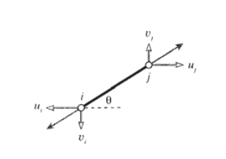
where \(u\) and \(v\) are the horizontal and vertical components of the deflections, respectively. (The displacements at node \(i\) drawn in Figure 12 are negative.) This relation can be written in matrix form as:
\[\delta = \begin{bmatrix} -c & -s & c & s \end{bmatrix} \left \{ \begin{matrix} u_i \\ v_i \\ u_j \\ v_j \end{matrix} \right \}\nonumber \]
Here \(c = \cos \theta\) and \(s = \sin \theta\).
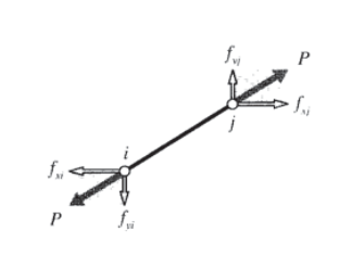
The axial force P that accompanies the elongation \(\delta\) is given by Hooke’s law for linear elastic bodies as \(P = (AE/L)\delta\). The horizontal and vertical nodal forces are shown in Figure 13; these can be written in terms of the total axial force as:
\[\left \{ \begin{matrix} f_{xi} \\ f_{yi} \\ f_{xj} \\ f_{yj} \end{matrix} \right \} = \left \{ \begin{matrix} -c \\ -s \\ c \\ s \end{matrix} \right \} P = \left \{ \begin{matrix} -c \\ -s \\ c \\ s \end{matrix} \right \} \dfrac{AE}{L} \delta\nonumber \]
\[\left \{ \begin{matrix} -c \\ -s \\ c \\ s \end{matrix} \right \} \dfrac{AE}{L} \begin{bmatrix} -c & -s & c & s \end{bmatrix} \left \{ \begin{matrix} u_i \\ v_i \\ u_j \\ v_j \end{matrix} \right \}\nonumber \]
Carrying out the matrix multiplication:
\[\left \{ \begin{matrix} f_{xi} \\ f_{yi} \\ f_{xj} \\ f_{yj} \end{matrix} \right \} = \dfrac{AE}{L} \begin{bmatrix} c^2 & cs & -c^2 & -cs \\ cs & s^2 & -cs & -s^2 \\ -c^2 & -cs & c^2 & cs \\ -cs & -s^2 & cs & s^2 \end{bmatrix} \left \{ \begin{matrix} u_i \\ v_i \\ u_j \\ v_j \end{matrix} \right \} \nonumber \]
The quantity in brackets, multiplied by \(AE/L\), is known as the "element stiffness matrix" \(k_{ij}\). Each of its terms has a physical significance, representing the contribution of one of the displacements to one of the forces. The global system of equations is formed by combining the element stiffness matrices from each truss element in turn, so their computation is central to the method of matrix structural analysis. The principal difference between the matrix truss method and the general finite element method is in how the element stiffness matrices are formed; most of the other computer operations are the same.
Assembly of multiple element contributions
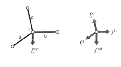
The next step is to consider an assemblage of many truss elements connected by pin joints. Each element meeting at a joint, or node, will contribute a force there as dictated by the displacements of both that element’s nodes (see Figure 14). To maintain static equilibrium, all element force contributions \(f_i^{elem}\) at a given node must sum to the force \(f_i^{ext}\) that is externally applied at that node:
\[f_i^{ext} = \sum_{elem} f_i^{elem} = (\sum_{elelm} k_{ij}^{elem} u_j) = (\sum_{elem} k_{ij}^{elem}) u_j = K_{ij} u_j\nonumber \]
Each element stiffness matrix \(k_{ij}^{elem}\) is added to the appropriate location of the overall, or "global" stiffness matrix \(K_{ij}\) that relates all of the truss displacements and forces. This process is called "assembly." The index numbers in the above relation must be the "global" numbers assigned to the truss structure as a whole. However, it is generally convenient to compute the individual element stiffness matrices using a local scheme, and then to have the computer convert to global numbers when assembling the individual matrices.
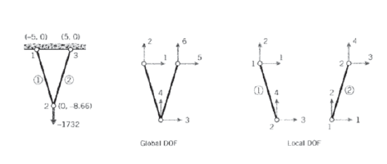
The assembly process is at the heart of the finite element method, and it is worthwhile to do a simple case by hand to see how it really works. Consider the two-element truss problem of Figure 7, with the nodes being assigned arbitrary "global" numbers from 1 to 3. Since each node can in general move in two directions, there are 3 \(\times\) 2 = 6 total degrees of freedom in the problem. The global stiffness matrix will then be a 6 \(\times\) 6 array relating the six displacements to the six externally applied forces. Only one of the displacements is unknown in this case, since all but the vertical displacement of node 2 (degree of freedom number 4) is constrained to be zero. Figure 15 shows a workable listing of the global numbers, and also "local" numbers for each individual element.
Using the local numbers, the 4 \(\times\) 4 element stiffness matrix of each of the two elements can be evaluated according to Equation 2.1.10. The inclination angle is calculated from the nodal coordinates as
\[\theta = \tan^{-1} \dfrac{y_2 -y_1}{x_2 - x_1}\nonumber \]
The resulting matrix for element 1 is:
\[k^{(1)} = \begin{bmatrix} 25.00 & -43.30 & -25.00 & 43.30 \\ -43.30 & 75.00 & 43.30 & -75.00 \\ -25.00 & 43.30 & 25.00 & -43.30 \\ 43.30 & -75.00 & -43.30 & 75.00 \end{bmatrix} \times 10^3\nonumber \]
and for element 2:
\[k^{(2)} = \begin{bmatrix} 25.00 & 43.30 & -25.00 & -43.30 \\ 43.30 & 75.00 & -43.30 & -75.00 \\ -25.00 & -43.30 & 25.00 & 43.30 \\ -43.30 & -75.00 & 43.30 & 75.00 \end{bmatrix} \times 10^3\nonumber \]
(It is important the units be consistent; here lengths are in inches, forces in pounds, and moduli in psi. The modulus of both elements is \(E = 10\) Mpsi and both have area \(A = 0.1\ in^2\).) These matrices have rows and columns numbered from 1 to 4, corresponding to the local degrees of freedom of the element. However, each of the local degrees of freedom can be matched to one of the global degrees of the overall problem. By inspection of Figure 15, we can form the following table that maps local to global numbers:
| local | global, element 1 | global, element 2 |
| 1 | 1 | 3 |
| 2 | 2 | 4 |
| 3 | 3 | 4 |
| 4 | 4 | 6 |
Using this table, we see for instance that the second degree of freedom for element 2 is the fourth degree of freedom in the global numbering system, and the third local degree of freedom corresponds to the fifth global degree of freedom. Hence the value in the second row and third column of the element stiffness matrix of element 2, denoted \(k_{23}^{(2)}\), should be added into the position in the fourth row and fifth column of the 6 \(\times\) 6 global stiffness matrix. We write this as
\[k_{23}^{(2)} \to K_{4,5}\nonumber \]
Each of the sixteen positions in the stiffness matrix of each of the two elements must be added into the global matrix according to the mapping given by the table. This gives the result
\[K = \begin{bmatrix} k_{11}^{(1)} & k_{12}^{(1)} & k_{13}^{(1)} & k_{14}^{(1)} & 0 & 0 \\ k_{21}^{(1)} & k_{22}^{(1)} & k_{23}^{(1)} & k_{24}^{(1)} & 0 & 0 \\ k_{31}^{(1)} & k_{32}^{(1)} & k_{33}^{(1)} + k_{11}^{(2)} & k_{34}^{(1)} + k_{12}^{(2)} & k_{13}^{(2)} & k_{14}^{(2)} \\ k_{41}^{(1)} & k_{42}^{(1)} & k_{43}^{(1)} + k_{21}^{(2)} & k_{44}^{(1)} + k_{22}^{(2)} & k_{23}^{(2)} & k_{24}^{(2)} \\ 0 & 0 & k_{31}^{(2)} & k_{32}^{(2)} & k_{33}^{(2)} & k_{34}^{(2)} \\ 0 & 0 & k_{41}^{(2)} & k_{42}^{(2)} & k_{43}^{(2)} & k_{44}^{(2)} \end{bmatrix}\nonumber \]
This matrix premultiplies the vector of nodal displacements according to Equation 2.1.9 to yield the vector of externally applied nodal forces. The full system equations, taking into account the known forces and displacements, are then
\[10^3 \begin{bmatrix} 25.0 & -43.3 & -25.0 & 43.0 & 0.0 & 0.00 \\ -43.3 & 75.0 & 43.3 & -75.0 & 0.0 & 0.00 \\ -25.0 & 43.3 & 50.0 & 0.0 & -25.0 & -43.30 \\ 43.3 & -75.0 & 0.0 & 150.0 & -43.3 & -75.00 \\ 0.0 & 0.0 & -25.0 & -43.3 & 25.0 & 43.30 \\ 0.0 & 0.0 & -43.3 & -75.0 & 43.3 & 75.00 \end{bmatrix} \left \{ \begin{array} 0 \\ 0 \\ 0 \\ u_4 \\ 0 \\ 0 \end{array} \right \} = \left \{ \begin{array} f_1 \\ f_2 \\ f_3 \\ -1732 \\ f_5 \\ f_5 \end{array} \right \}\nonumber \]
Note that either the force or the displacement for each degree of freedom is known, with the accompanying displacement or force being unknown. Here only one of the displacements (\(u_4\)) is unknown, but in most problems the unknown displacements far outnumber the unknown forces. Note also that only those elements that are physically connected to a given node can contribute a force to that node. In most cases, this results in the global stiffness matrix containing many zeroes corresponding to nodal pairs that are not spanned by an element. Effective computer implementations will take advantage of the matrix sparseness to conserve memory and reduce execution time.
In larger problems the matrix equations are solved for the unknown displacements and forces by Gaussian reduction or other techniques. In this two-element problem, the solution for the single unknown displacement can be written down almost from inspection. Multiplying out the fourth row of the system, we have
\[0 + 0 + 0 + 150 \times 10^3 u_4 + 0 + 0 = -1732\nonumber \]
\[u_4 = -1732/150 \times 10^3 = -0.01155 \ in\nonumber \]
Now any of the unknown forces can be obtained directly. Multiplying out the first row for instance gives
\[0 + 0 + 0 + (43.4) (-0.0115) \times 10^3 + 0 + 0 = f_1\nonumber \]
\[f_1 = -500 \ lb\nonumber \]
The negative sign here indicates the horizontal force on global node #1 is to the left, opposite the direction assumed in Figure 15.
The process of cycling through each element to form the element stiffness matrix, assembling the element matrix into the correct positions in the global matrix, solving the equations for displacements and then back-multiplying to compute the forces, and printing the results can be automated to make a very versatile computer code.
Larger-scale truss (and other) finite element analysis are best done with a dedicated computer code, and an excellent one for learning the method is available from the web at (https://web.archive.org/web/20060108...urceforge.net/). This code, named felt was authored by Jason Gobat and Darren Atkinson for educational use, and incorporates number of novel features to promote user-friendliness. Complete information describing this code, as well as the C-language source and a number of trial runs and auxiliary code module is available via their web pages. If you have access to X-window workstations, a graphical shell named velvet is available as well.
To illustrate how this code operates for a somewhat larger problem, consider the six-element truss of Figure 4, analyzed earlier both by the joint-at-a-time free body analysis approach and by Castigliano’s method. The truss is redrawn in Figure 16 by the velvet graphical interface.
The input dataset, which can be written manually or developed graphically in velvet, employs parsing techniques to simplify what can be a very tedious and error-prone step in finite element analysis. The dataset for this 6-element truss is:
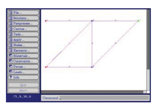
problem description
nodes=5 elements=6

nodes
1 x=0 y=100 z=0 constraint=pin
2 x=100 y=100 z=0 constraint=planar
3 x=200 y=100 z=0 force=P
4 x=0 y=0 z=0 constraint=pin
5 x=100 y=0 z=0 constraint=planar

truss elements
1  nodes=[1,2] material=steel
2  nodes=[2,3]
3  nodes=[4,2]
4  nodes=[2,5]
5  nodes=[5,3]
6  nodes=[4,5]

material properties
steel E=3e+07 A=0.5

distributed loads

constraints
free Tx=u Ty=u Tz=u Rx=u Ry=u Rz=u
pin Tx=c Ty=c Tz=c Rx=u Ry=u Rz=u
planar Tx=u Ty=u Tz=c Rx=u Ry=u Rz=u

forces
P Fy=-1000

end
The meaning of these lines should be fairly evident on inspection, although the felt documentation should be consulted for more detail. The output produced by felt for these data is:
**  **
Nodal Displacements
----------------------------------------------------------------
Node #    DOF 1      DOF 2    DOF 3    DOF 4    DOF 5    DOF 6
----------------------------------------------------------------
  1           0          0        0        0        0        0
  2    0.013333   -0.03219        0        0        0        0
  3        0.02  -0.084379        0        0        0        0
  4           0          0        0        0        0        0
  5  -0.0066667  -0.038856        0        0        0        0


Element Sress
-----------------------------------------------------
1:            4000
2:            2000
3:         -2828.4
4:            2000
5:         -2828.4
6:           -2000
Material Usage Summary
--------------------------
Material: steel
Number:   6
Length:   682.8427
Mass:     0.0000

Total mass: 0.0000
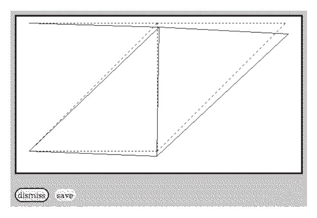
Note that the vertical displacement of node 3 (the DOF 2 value) is -0.0844, the same value obtained earlier in Example \(\PageIndex{3}\). Figure 17 shows the velvet graphical output for the truss deflections (greatly magnified).
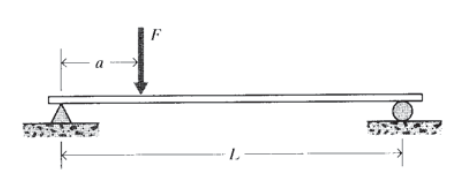
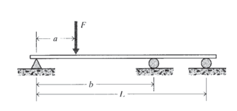
A rigid beam of length \(L\) rests on two supports that resist vertical motion, and is loaded by a vertical force \(F\) a distance a from the left support. Draw a free body diagram for
the beam, replacing the supports by the reaction forces \(R_1\) and \(R_2\) that they exert on the
beam. Solve for the reaction forces in terms of \(F, a\), and \(L\).
A third support is added to the beam of the previous problem. Draw the free-body diagram for this case, and write the equilibrium equations available to solve for the reaction forces at each support. Is it possible to solve for all the reaction forces?
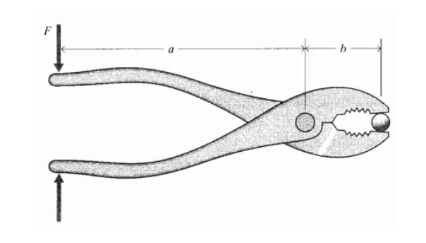
The handles of a pair of pliers are sqeezed with a force F. Draw a free-body diagram for one of the pliers’ arms. What is the force exerted on an object gripped between the pliers faces?
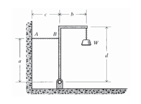
An object of weight \(W\) is suspended from a frame as shown. What is the tension in the retraining cable \(AB\)?
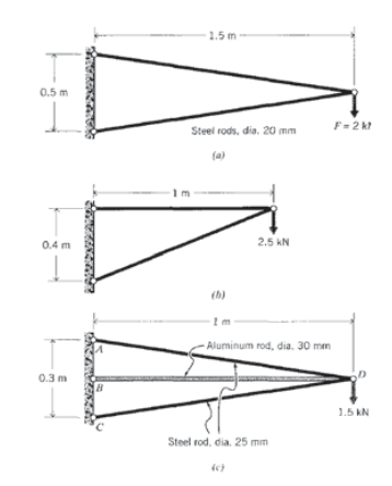
(a) - (h) Determine the force in each element of the trusses drawn below.
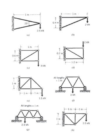
(a) - (h) Using geometrical considerations, determine the deflection of the loading point (the point at which the load is applied, in the direction of the load) for the trusses in Exercise \(\PageIndex{5}\). All elements are constructed of 20 mm diameter round carbon steel rods.
(a) - (h) Same as Exercise \(\PageIndex{6}\), but using Castigliano’s theorem.
(a) - (h) Same as \(\PageIndex{6}\, but using finite element analysis.
Find the element forces and deflection at the loading point for the truss shown, using the method of your own choice.
(a) - (c) Write out the global stiffness matrices for the trusses listed below, and solve for the unknown forces and displacements.
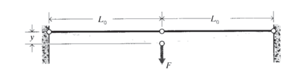
Two truss elements of equal initial length \(L_0\) are connected horizontally. Assuming the elements remain linearly elastic at all strains, determine the downward deflection \(y\) as a function of a load \(F\) applied transversely to the joint.