
2.3: Shear and Torsion
- Page ID
- 44533
\( \newcommand{\vecs}[1]{\overset { \scriptstyle \rightharpoonup} {\mathbf{#1}} } \)
\( \newcommand{\vecd}[1]{\overset{-\!-\!\rightharpoonup}{\vphantom{a}\smash {#1}}} \)
\( \newcommand{\dsum}{\displaystyle\sum\limits} \)
\( \newcommand{\dint}{\displaystyle\int\limits} \)
\( \newcommand{\dlim}{\displaystyle\lim\limits} \)
\( \newcommand{\id}{\mathrm{id}}\) \( \newcommand{\Span}{\mathrm{span}}\)
( \newcommand{\kernel}{\mathrm{null}\,}\) \( \newcommand{\range}{\mathrm{range}\,}\)
\( \newcommand{\RealPart}{\mathrm{Re}}\) \( \newcommand{\ImaginaryPart}{\mathrm{Im}}\)
\( \newcommand{\Argument}{\mathrm{Arg}}\) \( \newcommand{\norm}[1]{\| #1 \|}\)
\( \newcommand{\inner}[2]{\langle #1, #2 \rangle}\)
\( \newcommand{\Span}{\mathrm{span}}\)
\( \newcommand{\id}{\mathrm{id}}\)
\( \newcommand{\Span}{\mathrm{span}}\)
\( \newcommand{\kernel}{\mathrm{null}\,}\)
\( \newcommand{\range}{\mathrm{range}\,}\)
\( \newcommand{\RealPart}{\mathrm{Re}}\)
\( \newcommand{\ImaginaryPart}{\mathrm{Im}}\)
\( \newcommand{\Argument}{\mathrm{Arg}}\)
\( \newcommand{\norm}[1]{\| #1 \|}\)
\( \newcommand{\inner}[2]{\langle #1, #2 \rangle}\)
\( \newcommand{\Span}{\mathrm{span}}\) \( \newcommand{\AA}{\unicode[.8,0]{x212B}}\)
\( \newcommand{\vectorA}[1]{\vec{#1}} % arrow\)
\( \newcommand{\vectorAt}[1]{\vec{\text{#1}}} % arrow\)
\( \newcommand{\vectorB}[1]{\overset { \scriptstyle \rightharpoonup} {\mathbf{#1}} } \)
\( \newcommand{\vectorC}[1]{\textbf{#1}} \)
\( \newcommand{\vectorD}[1]{\overrightarrow{#1}} \)
\( \newcommand{\vectorDt}[1]{\overrightarrow{\text{#1}}} \)
\( \newcommand{\vectE}[1]{\overset{-\!-\!\rightharpoonup}{\vphantom{a}\smash{\mathbf {#1}}}} \)
\( \newcommand{\vecs}[1]{\overset { \scriptstyle \rightharpoonup} {\mathbf{#1}} } \)
\(\newcommand{\longvect}{\overrightarrow}\)
\( \newcommand{\vecd}[1]{\overset{-\!-\!\rightharpoonup}{\vphantom{a}\smash {#1}}} \)
\(\newcommand{\avec}{\mathbf a}\) \(\newcommand{\bvec}{\mathbf b}\) \(\newcommand{\cvec}{\mathbf c}\) \(\newcommand{\dvec}{\mathbf d}\) \(\newcommand{\dtil}{\widetilde{\mathbf d}}\) \(\newcommand{\evec}{\mathbf e}\) \(\newcommand{\fvec}{\mathbf f}\) \(\newcommand{\nvec}{\mathbf n}\) \(\newcommand{\pvec}{\mathbf p}\) \(\newcommand{\qvec}{\mathbf q}\) \(\newcommand{\svec}{\mathbf s}\) \(\newcommand{\tvec}{\mathbf t}\) \(\newcommand{\uvec}{\mathbf u}\) \(\newcommand{\vvec}{\mathbf v}\) \(\newcommand{\wvec}{\mathbf w}\) \(\newcommand{\xvec}{\mathbf x}\) \(\newcommand{\yvec}{\mathbf y}\) \(\newcommand{\zvec}{\mathbf z}\) \(\newcommand{\rvec}{\mathbf r}\) \(\newcommand{\mvec}{\mathbf m}\) \(\newcommand{\zerovec}{\mathbf 0}\) \(\newcommand{\onevec}{\mathbf 1}\) \(\newcommand{\real}{\mathbb R}\) \(\newcommand{\twovec}[2]{\left[\begin{array}{r}#1 \\ #2 \end{array}\right]}\) \(\newcommand{\ctwovec}[2]{\left[\begin{array}{c}#1 \\ #2 \end{array}\right]}\) \(\newcommand{\threevec}[3]{\left[\begin{array}{r}#1 \\ #2 \\ #3 \end{array}\right]}\) \(\newcommand{\cthreevec}[3]{\left[\begin{array}{c}#1 \\ #2 \\ #3 \end{array}\right]}\) \(\newcommand{\fourvec}[4]{\left[\begin{array}{r}#1 \\ #2 \\ #3 \\ #4 \end{array}\right]}\) \(\newcommand{\cfourvec}[4]{\left[\begin{array}{c}#1 \\ #2 \\ #3 \\ #4 \end{array}\right]}\) \(\newcommand{\fivevec}[5]{\left[\begin{array}{r}#1 \\ #2 \\ #3 \\ #4 \\ #5 \\ \end{array}\right]}\) \(\newcommand{\cfivevec}[5]{\left[\begin{array}{c}#1 \\ #2 \\ #3 \\ #4 \\ #5 \\ \end{array}\right]}\) \(\newcommand{\mattwo}[4]{\left[\begin{array}{rr}#1 \amp #2 \\ #3 \amp #4 \\ \end{array}\right]}\) \(\newcommand{\laspan}[1]{\text{Span}\{#1\}}\) \(\newcommand{\bcal}{\cal B}\) \(\newcommand{\ccal}{\cal C}\) \(\newcommand{\scal}{\cal S}\) \(\newcommand{\wcal}{\cal W}\) \(\newcommand{\ecal}{\cal E}\) \(\newcommand{\coords}[2]{\left\{#1\right\}_{#2}}\) \(\newcommand{\gray}[1]{\color{gray}{#1}}\) \(\newcommand{\lgray}[1]{\color{lightgray}{#1}}\) \(\newcommand{\rank}{\operatorname{rank}}\) \(\newcommand{\row}{\text{Row}}\) \(\newcommand{\col}{\text{Col}}\) \(\renewcommand{\row}{\text{Row}}\) \(\newcommand{\nul}{\text{Nul}}\) \(\newcommand{\var}{\text{Var}}\) \(\newcommand{\corr}{\text{corr}}\) \(\newcommand{\len}[1]{\left|#1\right|}\) \(\newcommand{\bbar}{\overline{\bvec}}\) \(\newcommand{\bhat}{\widehat{\bvec}}\) \(\newcommand{\bperp}{\bvec^\perp}\) \(\newcommand{\xhat}{\widehat{\xvec}}\) \(\newcommand{\vhat}{\widehat{\vvec}}\) \(\newcommand{\uhat}{\widehat{\uvec}}\) \(\newcommand{\what}{\widehat{\wvec}}\) \(\newcommand{\Sighat}{\widehat{\Sigma}}\) \(\newcommand{\lt}{<}\) \(\newcommand{\gt}{>}\) \(\newcommand{\amp}{&}\) \(\definecolor{fillinmathshade}{gray}{0.9}\)Introduction
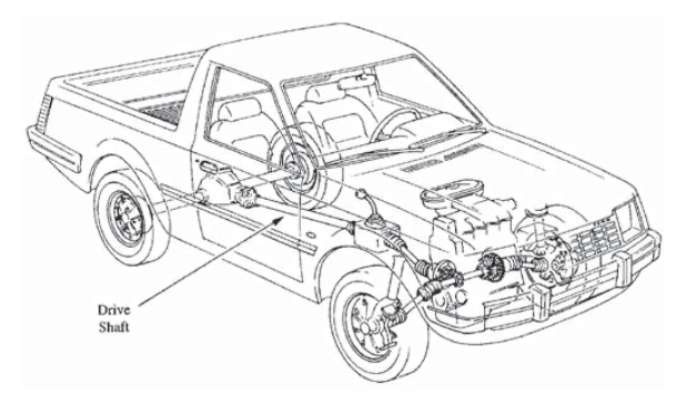
Torsionally loaded shafts are among the most commonly used structures in engineering. For instance, the drive shaft of a standard rear-wheel drive automobile, depicted in Figure 1, serves primarily to transmit torsion. These shafts are almost always hollow and circular in cross section, transmitting power from the transmission to the differential joint at which the rotation is diverted to the drive wheels. As in the case of pressure vessels, it is important to be aware of design methods for such structures purely for their inherent usefulness. However, we study them here also because they illustrate the role of shearing stresses and strains.
Shearing stresses and strains
Not all deformation is elongational or compressive, and we need to extend our concept of strain to include “shearing,” or “distortional,” effects. To illustrate the nature of shearing distortions, first consider a square grid inscribed on a tensile specimen as depicted in Figure 2(a). Upon uniaxial loading, the grid would be deformed so as to increase the length of the lines in the tensile loading direction and contract the lines perpendicular to the loading direction. However, the lines remain perpendicular to one another. These are termed normal strains, since planes normal to the loading direction are moving apart.
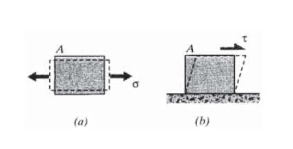
Now consider the case illustrated in Figure 2(b), in which the load \(P\) is applied transversely to the specimen. Here the horizontal lines tend to slide relative to one another, with line lengths of the originally square grid remaining unchanged. The vertical lines tilt to accommodate this motion, so the originally right angles between the lines are distorted. Such a loading is termed direct shear. Analogously to our definition of normal stress as force per unit area(See Module 1, Introduction to Elastic Response), or \(\sigma = P/A\), we write the shear stress \(\tau\) as
\[\tau = \dfrac{P}{A}\nonumber \]
This expression is identical to the expression for normal stress, but the different symbol \(\tau\) reminds us that the loading is transverse rather than extensional.
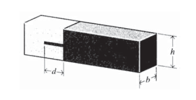
Two timbers, of cross-sectional dimension \(b \times h\), are to be glued together using a tongue-and-groove joint as shown in Figure 3, and we wish to estimate the depth \(d\) of the glue joint so as to make the joint approximately as strong as the timber itself.
The axial load \(P\) on the timber acts to shear the glue joint, and the shear stress in the joint is just the load divided by the total glue area:
\[\tau = \dfrac{P}{2bd}\nonumber \]
If the bond fails when \(\tau\) reaches a maximum value \(\tau_f\), the load at failure will be \(P_f = (2bd) \tau_f\). The load needed to fracture the timber in tension is \(P_f = bh \sigma_f\), where \(\sigma_f\) is the ultimate tensile strength of the timber. Hence if the glue joint and the timber are to be equally strong we have
\[(2bd) \tau_f = bh\sigma_f \to d = \dfrac{h\sigma_f}{2\tau_f}\nonumber \]
Normal stresses act to pull parallel planes within the material apart or push them closer together, while shear stresses act to slide planes along one another. Normal stresses promote crack formation and growth, while shear stresses underlie yield and plastic slip. The shear stress can be depicted on the stress square as shown in Figure 4(a); it is traditional to use a half-arrowhead to distinguish shear stress from normal stress. The \(yx\) subscript indicates the stress is on the \(y\) plane in the \(x\) direction.
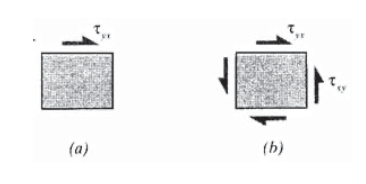
The \(\tau_{yx}\) arrow on the \(+y\) plane must be accompanied by one in the opposite direction on the \(-y\) plane, in order to maintain horizontal equilibrium. But these two arrows by themselves would tend to cause a clockwise rotation, and to maintain moment equilibrium we must also add two vertical arrows as shown in Figure 4(b); these are labeled \(\tau_{xy}\), since they are on \(x\) planes in the y direction. For rotational equilibrium, the magnitudes of the horizontal and vertical stresses must be equal:
\[\tau_{yx} = \tau_{xy} \nonumber \]
Hence any shearing that tends to cause tangential sliding of horizontal planes is accompanied by an equal tendency to slide vertical planes as well. Note that all of these are positive by our earlier convention of + arrows on + faces being positive. A positive state of shear stress, then, has arrows meeting at the upper right and lower left of the stress square. Conversely, arrows in a negative state of shear meet at the lower right and upper left.
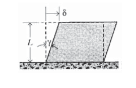
The strain accompanying the shear stress \(\tau_{xy}\) is a shear strain denoted \(\gamma_{xy}\). This quantity is a deformation per unit length just as was the normal strain \(\epsilon\), but now the displacement is transverse to the length over which it is distributed (see Figure 5). This is also the distortion or change in the right angle:
\[\dfrac{\delta}{L} = \tan \gamma \approx \gamma \nonumber \]
This angular distortion is found experimentally to be linearly proportional to the shear stress at sufficiently small loads, and the shearing counterpart of Hooke’s Law can be written as
\[\tau_{xy} = G\gamma_{xy} \nonumber \]
where \(G\) is a material property called the shear modulus. for isotropic materials (properties same in all directions), there is no Poisson-type effect to consider in shear, so that the shear strain is not influenced by the presence of normal stresses. Similarly, application of a shearing stress has no influence on the normal strains. For plane stress situations (no normal or shearing stress components in the \(z\) direction), the constitutive equations as developed so far can be written:
\[\begin{array} {c} {\epsilon_x = \dfrac{1}{E} (\sigma_x - \nu \sigma_y)} \\ {\epsilon_y = \dfrac{1}{E} (\sigma_y - \nu \sigma_x)} \\ {\gamma_{xy} = \dfrac{1}{G} \tau_{xy}} \end{array} \nonumber \]
It will be shown later that for isotropic materials, only two of the material constants here are independent, and that
\[G = \dfrac{E}{2(1 + \nu)} \nonumber \]
Hence if any two of the three properties \(E, G\), or \(\nu\), are known, the other is determined.
Statics - Twisting Moments
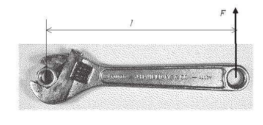
Twisting moments, or torques, are forces acting through distances (“lever arms”) so as to pro- mote rotation. The simple example is that of using a wrench to tighten a nut on a bolt as shown in Figure 6: if the bolt, wrench, and force are all perpendicular to one another, the moment is just the force F times the length l of the wrench: \(T = F \cdot l\). This relation will suffice when the geometry of torsional loading is simple as in this case, when the torque is applied “straight”.
Often, however, the geometry of the applied moment is a bit more complicated. Consider a not-uncommon case where for instance a spark plug must be loosened and there just isn’t room to put a wrench on it properly. Here a swiveled socket wrench might be needed, which can result in the lever arm not being perpendicular to the spark plug axis, and the applied force (from your hand) not being perpendicular to the lever arm. Vector algebra can make the geometrical calculations easier in such cases. Here the moment vector around a point \(O\) is obtained by crossing the vector representation of the lever arm \(r\) from \(O\) with the force vector \(F\):
\[T = r \times F \nonumber \]
This vector is in a direction given by the right hand rule, and is normal to the plane containing the point \(O\) and the force vector. The torque tending to loosen the spark plug is then the component of this moment vector along the plug axis:
\[T = i \cdot (r \times F) \nonumber \]
where \(i\) is a unit vector along the axis. The result, a torque or twisting moment around an axis, is a scalar quantity.
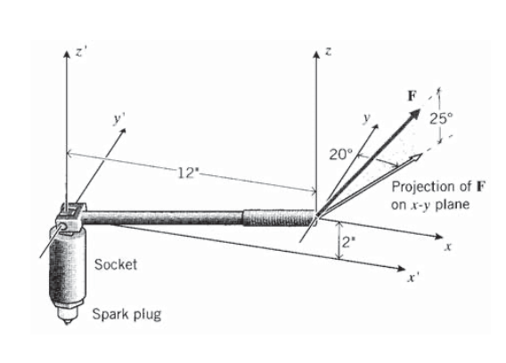
We wish to find the effective twisting moment on a spark plug, where the force applied to a swivel wrench that is skewed away from the plug axis as shown in Figure 7. An \(x'y'z'\) Cartesian coordinate system is established with \(z'\) being the spark plug axis; the free end of the wrench is \(2''\) above the \(x'y'\) plane perpendicular to the plug axis, and \(12''\) away from the plug along the \(x'\) axis. A 15 lb force is applied to the free end at a skewed angle of 25\(^{\circ}\) vertical and 20\(^{\circ}\) horizontal.
The force vector applied to the free end of the wrench is
\[F = 15 (\cos 25 \sin 20 i + \cos 25 \cos 20 j + \sin 25 k)\nonumber \]
The vector from the axis of rotation to the applied force is
\[r = 12 i + 0j + 2k \nonumber \]
where \(i,j,k\), are the unit vectors along the \(x, y, z\) axes. The moment vector around the point \(O\) is then
\[T_O = r\times F = (-25.55 i - 66.77j + 153.3k)\nonumber \]
and the scalar moment along the axis \(z'\) is
\[T_{z'} = k \cdot (r \times F) = 153.3 \ in - lb\nonumber \]
This is the torque that will loosen the spark plug, if you’re luckier than I am with cars.
Shafts in torsion are used in almost all rotating machinery, as in our earlier example of a drive shaft transmitting the torque of an automobile engine to the wheels. When the car is operating at constant speed (not accelerating), the torque on a shaft is related to its rotational speed \(\omega\) and the power \(W\) being transmitted:
\[W = T \omega \nonumber \]
Geared transmissions are usually necessary to keep the engine speed in reasonable bounds as the car speeds up, and the gearing must be considered in determining the torques applied to the shafts.
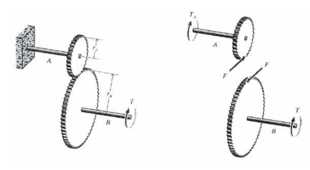
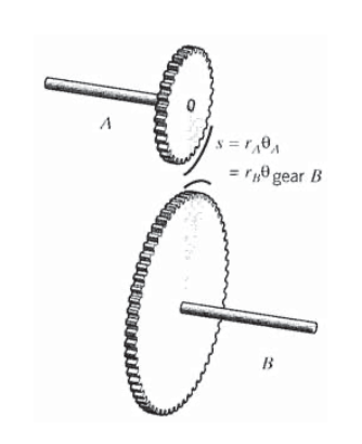
Consider a simple two-shaft gearing as shown in Figure 8, with one end of shaft \(A\) clamped and the free end of shaft \(B\) loaded with a moment \(T\). Drawing free-body diagrams for the two shafts separately, we see the force \(F\) transmitted at the gear periphery is just that which keeps shaft \(B\) in rotational equilibrium:
\[F \cdot r_B = T\nonumber \]
This same force acts on the periphery of gear \(A\), so the torque \(T_A\) experienced by shaft \(A\) is
\[T_A = F \cdot r_A = T \cdot \dfrac{r_A}{r_B}\nonumber \]
Torsional Stresses and Displacements
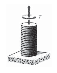
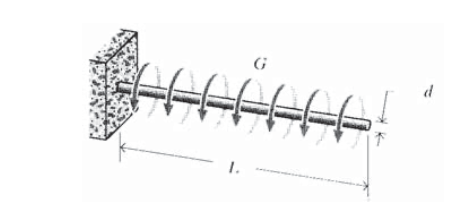
The stresses and deformations induced in a circular shaft by a twisting moment can be found by what is sometimes called the direct method of stress analysis. Here an expression of the geometrical form of displacement in the structure is proposed, after which the kinematic, constitutive, and equilibrium equations are applied sequentially to develop expressions for the strains and stresses. In the case of simple twisting of a circular shaft, the geometric statement is simply that the circular symmetry of the shaft is maintained, which implies in turn that plane cross sections remain plane, without warping. As depicted in Figure 9, the deformation is like a stack of poker chips that rotate relative to one another while remaining flat. The sequence of direct analysis then takes the following form:
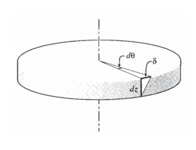
1. Geometrical statement: To quantify the geometry of deformation, consider an increment of length \(dz\) from the shaft as seen in Figure 10, in which the top rotates relative to the bottom by an increment of angle \(d\theta\). The relative tangential displacement of the top of a vertical line drawn at a distance \(r\) from the center is then:
\[\delta = r\ d\theta \nonumber \]
2. Kinematic or strain-displacement equation: The geometry of deformation fits exactly our earlier description of shear strain, so we can write:
\[\gamma_{z\theta} = \dfrac{\delta}{dz} = r \dfrac{d\theta}{dz} \nonumber \]
The subscript indicates a shearing of the \(z\) plane (the plane normal to the \(z\) axis) in the \(\theta\) direction. As with the shear stresses, \(\gamma_{z\theta} = \gamma_{\theta z}\), so the order of subscripts is arbitrary.
3. Constitutive equation: If the material is in its linear elastic regime, the shear stress is given directly from Hooke’s Law as:
\[\tau_{\theta z} = G\gamma_{\theta z} = Gr\dfrac{d \theta}{dz} \nonumber \]
The sign convention here is that positive twisting moments (moment vector along the +\(z\) axis) produce positive shear stresses and strains. However, it is probably easier simply to intuit in which direction the applied moment will tend to slip adjacent horizontal planes. Here the upper (+\(z\)) plane is clearly being twisted to the right relative to the lower (-\(z\)) plane, so the upper arrow points to the right. The other three arrows are then determined as well.
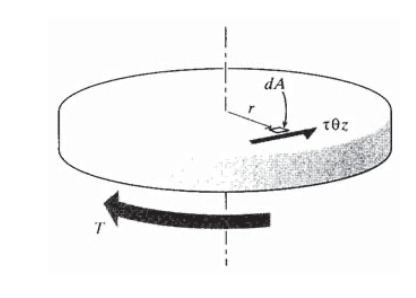
4. 4. Equilibrium equation: In order to maintain rotational equilibrium, the sum of the moments contributed by the shear stress acting on each differential area \(dA\) on the cross section must balance the applied moment \(T\) as shown in Figure 11:
\[T = \int_A \tau_{\theta z} r dA = \int_A Gr \dfrac{d\theta}{dz} rdA = G \dfrac{d \theta}{dz} \int_A r^2 d A\nonumber \]
The quantity \(\int r^2 dA\) is the polar moment of inertia \(J\), which for a hollow circular cross section is calculated as
\[J = \int_{R_i}^{R_o} r^2 2\pi r dr = \dfrac{\pi (R_o^4 - R_i^4)}{2} \nonumber \]
where \(R_i\) and \(R_o\) are the inside and outside radii. For solid shafts, \(R_i = 0\). The quantity \(d \theta /dz\) can now be found as
\[\dfrac{d\theta}{dz} = \dfrac{T}{GJ} \to \theta = \int_z \dfrac{T}{JG} dz\nonumber \]
Since in the simple twisting case under consideration the quantities \(T,J,G\) are constant along \(z\), the angle of twist can be written as
\[\dfrac{d\theta}{dz} = \text{constant} = \dfrac{\theta}{L}\nonumber \]
\[\theta = \dfrac{TL}{GJ} \nonumber \]
This is analogous to the expression \(\delta = PL/AE\) for the elongation of a uniaxial tensile specimen.
5. An explicit formula for the stress can be obtained by using this in Equation 2.3.11:
\[\tau_{\theta z} = Gr \dfrac{d\theta}{dz} = Gr \dfrac{\theta}{L} = \dfrac{Gr}{L} \dfrac{TL}{GJ}\nonumber \]
\[\tau_{\theta z} = \dfrac{Tr}{J} \nonumber \]
Note that the material property \(G\) has canceled from this final expression for stress, so that the the stresses are independent of the choice of material. Earlier, we have noted that stresses are independent of materials properties in certain pressure vessels and truss elements, and this was due to those structures being statically determinate. The shaft in torsion is not statically indeterminate, however; we had to use geometrical considerations and a statement of material linear elastic response as well as static equilibrium in obtaining the result. Since the material properties do not appear in the resulting equation for stress, it is easy to forget that the derivation depended on geometrical and material linearity. It is always important to keep in mind the assumptions used in derivations such as this, and be on guard against using the result in instances for which the assumptions are not justified.
For instance, we might twist a shaft until it breaks at a final torque of \(T = T_f\), and then use Equation 2.3.14 to compute an apparent ultimate shear strength: \(\tau_f = T_f r/J\). However, the material may very well have been stressed beyond its elastic limit in this test, and the assumption of material linearity may not have been valid at failure. The resulting value of \(\tau_f\) obtained from the elastic analysis is therefore fictitious unless proven otherwise, and could be substantially different than the actual stress. The fictitious value might be used, however, to estimate failure torques in shafts of the same material but of different sizes, since the actual failure stress would scale with the fictitious stress in that case. The fictitious failure stress calculated using the elastic analysis is often called the modulus of rupture in torsion.
Equation 2.3.14 shows one reason why most drive shafts are hollow, since there isn’t much point in using material at the center where the stresses are zero. Also, for a given quantity of material the designer will want to maximize the moment of inertia by placing the material as far from the center as possible. This is a powerful tool, since J varies as the fourth power of the radius.
An automobile engine is delivering 100 hp (horsepower) at 1800 rpm (revolutions per minute) to the drive shaft, and we wish to compute the shearing stress. From Equation 2.3.8, the torque on the shaft is
\[T = \dfrac{W}{\omega} = \dfrac{100\ hp (\tfrac{1}{1.341 \times 10^{-3}})\tfrac{N \cdot m}{s \cdot hp}}{1800 \tfrac{rev}{min} 2\pi \tfrac{rad}{rev} (\tfrac{1}{60}) \tfrac{min}{s}} = 396 N \cdot m\nonumber \]
The present drive shaft is a solid rod with a circular cross section and a diameter of \(d = 10\) mm. Using Equation 2.3.14, the maximum stress occurs at the outer surface of the rod as is
\[\tau_{\theta z} = \dfrac{Tr}{J}, r = d/2, J = \pi (d/2)^4/2\nonumber \]
\[\tau_{\theta z} = 252 \text{ MPa}\nonumber \]
Now consider what the shear stress would be if the shaft were made annular rather than solid, keeping the amount of material the same. The outer-surface shear stress for an annular shaft with outer radius \(r_o\) and inner radius \(r_i\) is
\[\tau_{\theta z} = \dfrac{T_{r_o}}{J}, J = \dfrac{\pi}{2} (r_o^4 - r_i^4)\nonumber \]
To keep the amount of material in the annular shaft the same as in the solid one, the cross-sectional areas must be the same. Since the cross-sectional area of the solid shaft is \(A_0 = \pi r^2\), the inner radius \(r_i\) of an annular shaft with outer radius ro and area \(A_0\) is found as
\[A_0 = \pi (r_o^2 - r_i^2) \to r_i = \sqrt{r_o^2 - (A_0/\pi)}\nonumber \]
Evaluating these equations using the same torque and with \(r_o = 30\) mm, we find \(r_i = 28.2\) mm (a 1.8 mm wall thickness) and a stress of \(\tau_{\theta z} = 44.5\) MPa. This is an 82% reduction in stress. The value of \(r\) in the elastic shear stress formula went up when we went to the annular rather than solid shaft, but this was more than offset by the increase in moment of inertia \(J\), which varies as \(r^4\).
Just as with trusses, the angular displacements in systems of torsion rods may be found from direct geometrical considerations. In the case of the two-rod geared system described earlier, the angle of twist of rod \(A\) is
\[\theta_A = (\dfrac{L}{GJ})_A T_A = (\dfrac{L}{GJ})_A T \cdot \dfrac{r_A}{r_B}\nonumber \]
This rotation will be experienced by gear \(A\) as well, so a point on its periphery will sweep through an arc \(S\) of
\[S = \theta_A r_A = (\dfrac{L}{GJ})_A T \cdot \dfrac{r_A}{r_B} \cdot r_A \nonumber \]
Since gears \(A\) and \(B\) are connected at their peripheries, gear \(B\) will rotate through an angle of
\[\theta_{gear} B = \dfrac{S}{r_B} = (\dfrac{L}{GJ})_A \cdot \dfrac{r_A}{r_B} \cdot \dfrac{r_A}{r_B}\nonumber \]
(See Figure 11). Finally, the total angular displacement at the end of rod \(B\) is the rotation of gear \(B\) plus the twist of rod \(B\) itself:
\[\theta = \theta_{gear B} + \theta_{rod B} = (\dfrac{L}{GJ})_A T (\dfrac{r_A}{r_B})^2 + (\dfrac{L}{GJ})_B T\nonumber \]
Energy method for rotational displacement
The angular deformation may also be found using Castigliano’s Theorem(Castigliano’s Theorem is introduced in the Module 5, Trusses.), and in some problems this approach may be easier. The strain energy per unit volume in a material subjected to elastic shearing stresses \(\tau\) and strains \(\gamma\) arising from simple torsion is:
\[U^* = \int \tau d\gamma = \dfrac{1}{2} \tau \gamma = \dfrac{\tau^2}{2G} = \dfrac{1}{2G} (\dfrac{Tr}{J})^2\nonumber \]
This is then integrated over the specimen volume to obtain the total energy:
\[U = \int_V U^* dV = \int_L \int_A = \int_{L} \int_A \dfrac{1}{2G} (\dfrac{Tr}{J})^2 dA dz = \int_L \dfrac{T^2}{2GJ^2} \int_A r^2 dA\nonumber \]
\[U = \int_L \dfrac{T^2}{2GJ} dz \nonumber \]
If \(T, G, and J\) are constant along the length \(z\), this becomes simply
\[U = \dfrac{T^2L}{2GJ} \nonumber \]
which is analogous to the expression \(U = P^2L/2AE\) for tensile specimens.
In torsion, the angle \(\theta\) is the generalized displacement congruent to the applied moment \(T\), so Castigliano’s theorem is applied for a single torsion rod as
\[\theta = \dfrac{\partial U}{\partial T} = \dfrac{TL}{GJ}\nonumber \]
as before.
Consider the two shafts geared together discussed earlier (Figure 11). The energy method requires no geometrical reasoning, and follows immediately once the torques transmitted by the two shafts is known. Since the torques are constant along the lengths, we can write
\[U = \sum_i (\dfrac{T^2L}{2GJ})_i = (\dfrac{L}{2GJ})_A (T \dfrac{r_A}{r_B})^2 + (\dfrac{L}{2GJ})_B T^2\nonumber \]
\[\theta = \dfrac{\partial U}{\partial T} = (\dfrac{L}{GJ})_A (T \cdot \dfrac{r_A}{r_B}) (\dfrac{r_A}{r_B}) + (\dfrac{L}{GJ})_B T\nonumber \]
Noncircular sections: the Prandtl membrane analogy
Shafts with noncircular sections are not uncommon. Although a circular shape is optimal from a stress analysis view, square or prismatic shafts may be easier to produce. Also, round shafts often have keyways or other geometrical features needed in order to join them to gears. All of this makes it necessary to be able to cope with noncircular sections. We will outline one means of doing this here, partly for its inherent usefulness and partly to introduce a type of experimental stress analysis. Later modules will expand on these methods, and will present a more complete treatment of the underlying mathematical theory.
The lack of axial symmetry in noncircular sections renders the direct approach that led to Equation 2.3.14 invalid, and a thorough treatment must attack the differential governing equations of the problem mathematically. These equations will be discussed in later modules, but suffice it to say that they can be difficult to solve in closed form for arbitrarily shaped cross sections. The advent of finite element and other computer methods to solve these equations numerically has removed this difficulty to some degree, but one important limitation of numerical solutions is that they usually fail to provide intuitive insight as to why the stress distributions are the way they are: they fail to provide hints as to how the stresses might be modified favorably by design changes, and this intuition is one of the designer’s most important tools.
In an elegant insight, Prandtl(Ludwig Prandtl (1875–1953) is best known for his pioneering work in aerodynamics.) pointed out that the stress distribution in torsion can be described by a “Poisson” differential equation, identical in form to that describing the deflection of a flexible membrane supported and pressurized from below(J.P. Den Hartog, Advanced Strength of Materials, McGraw-Hill, New York, 1952). This provides the basis of the Prandtl membrane analogy, which was used for many years to provide a form of experimental stress analysis for noncircular shafts in torsion. Although this experimental use has been supplanted by the more convenient computer methods, the analogy provides a visualization of torsionally induced stresses that can provide the sort of design insight we seek.
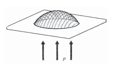
The analogy works such that the shear stresses in a torsionally loaded shaft of arbitrary cross section are proportional to the slope of a suitably inflated flexible membrane. The membrane is clamped so that its edges follow a shape similar to that of the noncircular section, and then displaced by air pressure. Visualize a horizontal sheet of metal with a circular hole in it, a sheet of rubber placed below the hole, and the rubber now made to bulge upward by pressure acting from beneath the plate (see Figure 13). The bulge will be steepest at the edges and horizontal at its center; i.e. its slope will be zero at the center and largest at the edges, just as the stresses in a twisted circular shaft.
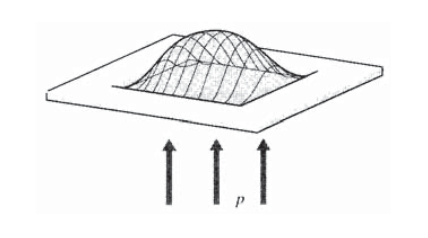
It is not difficult to visualize that if the hole were square as in Figure 14 rather than round, the membrane would be forced to lie flat (have zero slope) in the corners, and would have the steepest slopes at the midpoints of the outside edges. This is just what the stresses do. One good reason for not using square sections for torsion rods, then, is that the corners carry no stress and are therefore wasted material. The designer could remove them without consequence, the decision just being whether the cost of making circular rather than square shafts is more or less than the cost of the wasted material. To generalize the lesson in stress analysis, a protruding angle is not dangerous in terms of stress, only wasteful of material.
But conversely, an entrant angle can be extremely dangerous. A sharp notch cut into the shaft is like a knife edge cutting into the rubber membrane, causing the rubber to be almost vertical. Such notches or keyways are notorious stress risers, very often acting as the origination sites for fatigue cracks. They may be necessary in some cases, but the designer must be painfully aware of their consequences.
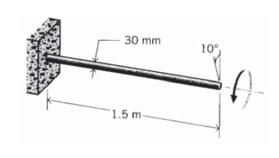
A torsion bar 1.5 m in length and 30 mm in diameter is clamped at one end, and the free end is twisted through an angle of 10 . Find the maximum torsional shear stress induced in the bar.
The torsion bar of Exercise \(\PageIndex{1}\) fails when the applied torque is 1500 N-m. What is the modulus of rupture in torsion? Is this the same as the material’s maximum shear stress?
A solid steel drive shaft is to be capable of transmitting 50 hp at 500 rpm. What should its diameter be if the maximum torsional shear stress is to be kept less that half the tensile yield strength?
How much power could the shaft of Prob. 3 transmit (at the same maximum torsional shear stress) if the same quantity of material were used in an annular rather than a solid shaft? Take the inside diameter to be half the outside diameter.
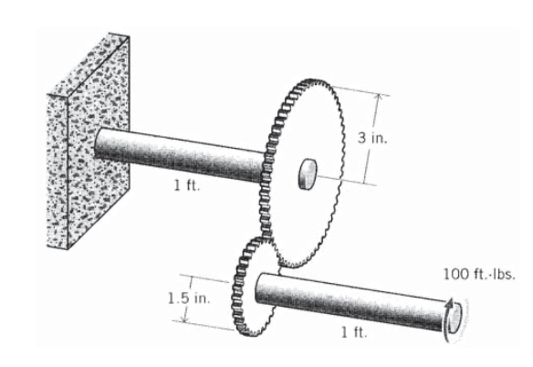
Two shafts, each 1 ft long and 1 in diameter, are connected by a 2:1 gearing, and the free end is loaded with a 100 ft-lb torque. Find the angle of twist at the loaded end.
A shaft of length \(L\), diameter \(d\), and shear modulus \(G\) is loaded with a uniformly distributed twisting moment of \(T_0\) (N-m/m). (The twisting moment \(T(x)\) at a distance \(x\) from the free end is therefore \(T_0x\).) Find the angle of twist at the free end.
A composite shaft 3 ft in length is constructed by assembling an aluminum rod, 2 in diameter, over which is bonded an annular steel cylinder of 0.5 in wall thickness. Determine the maximum torsional shear stress when the composite cylinder is subjected to a torque of 10,000 in-lb.
Sketch the shape of a membrane inflated through a round section containing an entrant keyway shape.