4.3: Beam Displacements

Introduction

We want to be able to predict the deflection of beams in bending, because many applications have limitations on the amount of deflection that can be tolerated. Another common need for deflection analysis arises from materials testing, in which the transverse deflection induced by a bending load is measured. If we know the relation expected between the load and the deflection, we can "back out" the material properties (specifically the modulus) from the measurement. We will show, for instance, that the deflection at the midpoint of a beam subjected to "three-point bending" (beam loaded at its center and simply supported at its edges) is

\(\delta_P = \dfrac{PL^3}{48EI}\)

where the length \(L\) and the moment of inertia \(I\) are geometrical parameters. If the ratio of \(\delta_P\) to \(P\) is measured experimentally, the modulus \(E\) can be determined. A stiffness measured this way is called the flexural modulus.

There are a number of approaches to the beam deflection problem, and many texts spend a good deal of print on this subject. The following treatment outlines only a few of the more straightforward methods, more with a goal of understanding the general concepts than with developing a lot of facility for doing them manually. In practice, design engineers will usually consult handbook tabulations of deflection formulas as needed, so even before the computer age many of these methods were a bit academic.

Multiple integration

In Module 12, we saw how two integrations of the loading function \(q(x)\) produces first the shear function \(V(x)\) and then the moment function \(M(x)\):

\[V = - \int q(x) dx + c_1\]

\[M = - \int V(x) dx + c_2\]

where the constants of integration \(c_1\) and \(c_2\) are evaluated from suitable boundary conditions on \(V\) and \(M\). (If singularity functions are used, the boundary conditions are included explicitly and the integration constants \(c_1\) and \(c_2\) are identically zero.) From Equation 6 in Module 13, the curvature \(v_{,xx} (x)\) is just the moment divided by the section modulus \(EI\). Another two integrations then give

\[v_{,x} (x) = \dfrac{1}{EI} \int M(x) dx + c_3\]

\[v(x) = \int v_{,x} (x) + c_4\]

where \(c_3\) and \(c_4\) are determined from boundary conditions on slope or deflection.

Example \(\PageIndex{1}\)

Figure 1: Three-point bending.

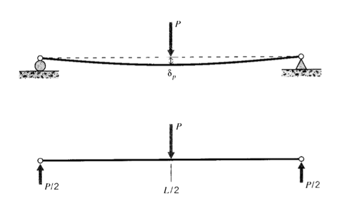
As an illustration of this process, consider the case of "three-point bending" shown in Figure 1. This geometry is often used in materials testing, as it avoids the need to clamp the specimen to the testing apparatus. If the load \(P\) is applied at the midpoint, the reaction forces at \(A\) and \(B\) are equal to half the applied load. The loading function is then

Integrating according to the above scheme:

\[\begin{array} {c} {V(x) = - \dfrac{P}{2} \langle x \rangle^0 + P \langle x - \dfrac{L}{2} \rangle^0} \\ {M(x) = \dfrac{P}{2} \langle x \rangle^1 - P \langle x - \dfrac{L}{2} \rangle^1} \\ {EIv_{,x} (x) = \dfrac{P}{4} \langle x \rangle^2 - \dfrac{P}{2} \langle x - \dfrac{L}{2} \rangle^2 + c_3} \end{array}\]

From symmetry, the beam has zero slope at the midpoint. Hence \(v_{,x} = 0 @ x = L/2\), so \(c_3\) can be found to be \(-PL^2/16\). Integrating again:

The deflection is zero at the left end, so \(c_4 = 0\). Rearranging, the beam deflection is given by

\[v = \dfrac{P}{48EI} [4x^3 - 3L^2x - 8 \langle x - \dfrac{L}{2} \rangle^3]\]

The maximum deflection occurs at \(x = L/2\), which we can evaluate just before the singularity term

\[\delta_{\max} = \dfrac{PL^3}{48EI}\]

This expression is much used in flexural testing, and is the example used to begin this module.

Before the loading function \(q(x)\) can be written, the reaction forces at the beam supports must be determined. If the beam is statically determinate, as in the above example, this can be done by invoking the equations of static equilibrium. Static determinacy means only two reaction forces or moments can be present, since we have only a force balance in the direction transverse to the beam axis and one moment equation available. A simply supported beam (one resting on only two supports) or a simply cantilevered beam are examples of such determinate beams; in the former case there is one reaction force at each support, and in the latter case there is one transverse force and one moment at the clamped end.

Of course, there is no stringent engineering reason to limit the number of beam supports to those sufficient for static equilibrium. Adding "extra" supports will limit deformations and stresses, and this will often be worthwhile in spite of the extra construction expense. But the analysis is now a bit more complicated, since not all of the unknown reactions can be found from the equations of static equilibrium. In these statically indeterminate cases it will be necessary to invoke geometrical constraints to develop enough equations to solve the problem.

This is done by writing the slope and deflection equations, carrying the unknown reaction forces and moments as undetermined parameters. The slopes and deflections are then set to their known values at the supports, and the resulting equations solved for the unknowns. If for instance a beam is resting on three supports, there will be three unknown reaction forces, and we will need a total of five equations: three for the unknown forces and two more for the constants of integration that arise when the slope and deflection equations are written. Two of these equations are given by static equilibrium, and three more are obtained by setting the deflections at the supports to zero. The following example illustrates the procedure, which is straightforward although tedious if done manually.

Example \(\PageIndex{2}\)

Consider a triply-supported beam of length \(L = 15\) as shown in Figure 2, carrying a constant uniform load of \(w = -10\). There are not sufficient equilibrium equations to determine the reaction forces \(R_a\), \(R_b\), and \(R_c\), so these are left as unknowns while multiple integration is used to develop a deflection equation:

Figure 2: Uniformly loaded beam resting on three supports.

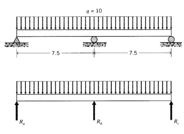
These equations have 5 unknowns: \(R_a, R_b, R_c, c_1\), and \(c_2\). These must be obtained from the two equilibrium equations

and the three known zero displacements at the supports

\(y(0) = y(L/2) = y(L) = 0\)

Although the process is straightforward, there is a lot of algebra to wade through. Statically indeterminate beams tend to generate tedious mathematics, but fortunately this can be reduced greatly by modern software. Follow how easily this example is handled by the Maple V package (some of the Maple responses removed for brevity):

> # read the library containing the Heaviside function
> readlib(Heaviside);
> # use the Heaviside function to define singularity functions;
> # sfn(x,a,n) is same is <x-a>^n
> sfn := proc(x,a,n) (x-a)^n * Heaviside(x-a) end; 
> # define the deflection function:
> y := (x)-> (Ra/6)*sfn(x,0,3)+(Rb/6)*sfn(x,7.5,3)+(Rc/6)*sfn(x,15,3)
>   -(10/24)*sfn(x,0,4)+c1*x+c2;
> # Now define the five constraint equations; first vertical equilibrium:
> eq1 := 0=Ra+Rb+Rc-(10*15);
> # rotational equilibrium:
> eq2 := 0=(10*15*7.5)-Rb*7.5-Rc*15;
> # Now the three zero displacements at the supports:
> eq3 := y(0)=0;
> eq4 := y(7.5)=0;
> eq5 := y(15)=0;
> # set precision; 4 digits is enough:
> Digits:=4;
> # solve the 5 equations for the 5 unknowns:
> solve({eq1,eq2,eq3,eq4,eq5},{Ra,Rb,Rc,c1,c2});
            {c2 = 0, c1 = -87.82, Rb = 93.78, Ra = 28.11, Rc = 28.11} 
> # assign the known values for plotting purposes:
> c1:=-87.82;c2:=0;Ra:=28.11;Rb:=93.78;Rc:=28.11;
> # the equation of the deflection curve is:
> y(x);
            3                                    3
4.686 x Heaviside(x) + 15.63 (x - 7.5) Heaviside(x - 7.5)
                    3                              4
        + 4.686 (x - 15) Heaviside(x - 15) - 5/12 x Heaviside(x) - 87.82 x
> # plot the deflection curve:
> plot(y(x),x=0..15);
> # The maximum deflection occurs at the quarter points: 
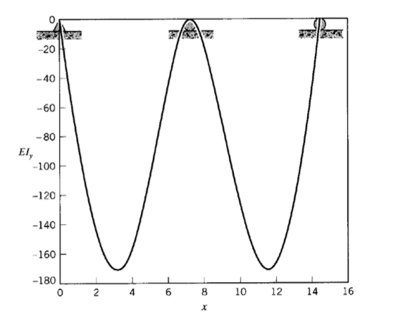
> y(15/4);
                                                -164.7 

The plot of the deflection curve is shown in Figure 3.

Figure 3: Deflection curve \(EIy(x)\) for uniformly loaded triply-supported beam (Note difference in horizontal and vertical scales).

Energy method

The strain energy in bending as given by Equation 8 of Module 13 can be used to find deflections, and this may be more convenient than successive integration if the deflection at only a single point is desired. Castigliano’s Theorem gives the deflection congruent to a load \(P\) as

\(\delta_P = \dfrac{\partial U}{\partial P} = \dfrac{\partial}{\partial P} \int_L \dfrac{M^2 dx}{2EI}\)

It is usually more convenient to do the differentiation before the integration, since this lowers the order of the expression in the integrand:

\(\delta P = \int_L \dfrac{M}{EI} \dfrac{\partial M}{\partial P} dx\)

where here \(E\) and \(I\) are assumed not to vary with \(x\).

The shear contribution to bending can be obtained similarly. Knowing the shear stress \(\tau = VQ/Ib\) (omitting the \(xy\) subscript on \(\tau\) for now), the strain energy due to shear \(U_s\) can be written

\(U_s = \int_V \dfrac{\tau^2}{2G} dV = \int_L \dfrac{V^2}{2GI} \left [\int_A \dfrac{Q^2}{L^2} dA \right ] dx\)

The integral over the cross-sectional area \(A\) is a purely geometrical factor, and we can write

\[U_s = \int_L \dfrac{V^2 f_s}{2GA} dA \]

where the \(f_s\) is a dimensionless form factor for shear defined as

\[f_s = \dfrac{A}{I^2} \int_A \dfrac{Q^2}{b^2} dA\]

Figure 4: Rectangular beam section.

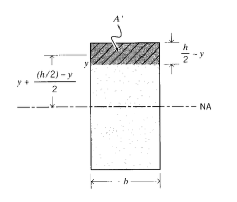
Evaluating \(f_s\) for rectangular sections for illustration (see Figure 4), we have in that case

\(A = bh, I = \dfrac{bh^3}{12}\)

\(f_s = \dfrac{(bh)}{(bh^3/12)^2} \int_{-h/2}^{h/2} \dfrac{1}{b^2} Q dy = \dfrac{6}{5}\)

Hence \(f_s\) is the same for all rectangular sections, regardless of their particular dimensions. Similarly, it can be shown (see Exercise \(\PageIndex{3}\)) that for solid circular sections \(f_s\) = 10/9 and for hollow circular sections \(f_s\) = 2.

Example \(\PageIndex{3}\)

If for instance we are seeking the deflection under the load \(P\) in the three-point bending example done earlier, we can differentiate the moment given in Equation 4.3.5 to obtain

Then

Expanding this and adjusting the limits of integration to account for singularity functions that have not been activated:

\(= -\dfrac{PL^3}{48EI}\)

as before.

The contribution of shear to the deflection can be found by using \(V = P/2\) in the equation for strain energy. For the case of a rectangular beam with \(f_s = 6/5\) we have:

\(U_s = \dfrac{(P/2)^2 (6/5)}{2GA}L\)

\(\delta_{P,s} = \dfrac{\partial U_s}{\partial P} = \dfrac{6PL}{20GA}\)

The shear contribution can be compared with the bending contribution by replacing \(A\) with \(12I/h^2\) (since \(A = bh\) and \(I = bh^3/12\)). Then the ratio of the shear to bending contributions is

\(\dfrac{PLh^2/40GI}{PL^3/24EI} = \dfrac{3h^2 E}{5L^2G}\)

Hence the importance of the shear term scales as (h/L)2, i.e. quadratically as the span-to-depth ratio.

The energy method is often convenient for systems having complicated geometries and com bined loading. For slender shafts transmitting axial, torsional, bending and shearing loads the strain energy is

\[U = \int_L \left (\dfrac{P^2}{2EA} + \dfrac{T^2}{2GJ} + \dfrac{M^2}{2EI} + \dfrac{V^2f_s}{2GA} \right ) dx\]

Example \(\PageIndex{4}\)

Consider a cantilevered circular beam as shown in Figure 5 that tapers from radius \(r_1\) to \(r_2\) over the length \(L\). We wish to determine the deflection caused by a force \(F\) applied to the free end of the beam, at an angle \(\theta\) from the horizontal. Turning to Maple to avoid the algebraic tedium, the dimensional parameters needed in Equation 4.3.10 are defined as:

Figure 5: Tapered circular beam.

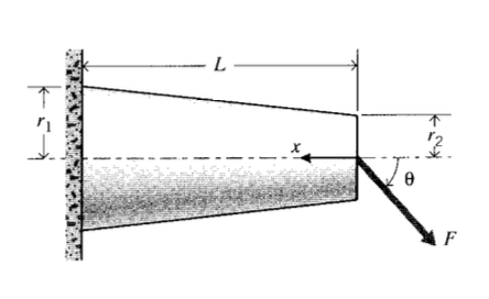
> r := proc (x) r1 + (r2-r1)*(x/L) end; 
> A := proc (r) Pi*(r(x))^2 end;
> Iz := proc (r) Pi*(r(x))^4 /4 end;
> Jp := proc (r) Pi*(r(x))^4 /2 end; 

where r(x) is the radius, A(r) is the section area, Iz is the rectangular moment of inertia, and Jp is the polar moment of inertia. The axial, bending, and shear loads are given in terms of \(F\) as

> P := F* cos(theta);
> V := F* sin(theta);
> M := proc (x) -F* sin(theta) * x end; 

The strain energies corresponding to tension, bending and shear are

> U1 := P^2/(2*E*A(r));
> U2 := (M(x))^2/(2*E*Iz(r));
> U3 := V^2*(10/9)/(2*G*A(r)); 
> U := int( U1+U2+U3, x=0..L); 

Finally, the deflection congruent to the load \(F\) is obtained by differentiating the total strain energy:

> dF := diff(U,F); 

The result of these manipulations yields

This displacement is in the direction of the applied force \(F\); the horizontal and vertical deflections of the end of the beam are then

\(\delta_x = \delta_F \cos \theta\)

\(\delta_y = \delta_F \sin \theta\)

Superposition

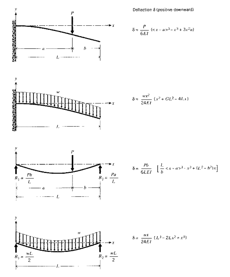
In practice, many beams will be loaded in a complicated manner consisting of several concentrated or distributed loads acting at various locations along the beam. Although these multiple-load cases can be solved from scratch using the methods described above, it is often easier to solve the problem by superposing solutions of simpler problems whose solutions are tabulated. Figure 6 gives an abbreviated collection of deflection formulas(A more exhaustive listing is available in W.C. Young, Roark’s Formulas for Stress and Strain, McGraw-Hill, New York, 1989.) that will suffice for many problems. The superposition approach is valid since the governing equations are linear; hence the response to a combination of loads is the sum of the responses that would be generated by each separate load acting alone.

Figure 6: Deflections for cantilevered and simply-supported beams, under concentrated and distributed loading.

Example \(\PageIndex{5}\)

Figure 7: Four-point bending.

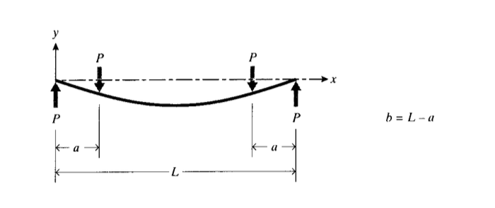
We wish to find the equation of the deflection curve for a simply-supported beam loaded in symmetric four-point bending as shown in Figure 7. From Figure 6, the deflection of a beam with a single load at a distance \(a\) from the left end is \(\delta (x) = \dfrac{Pb}{6LEI} [\dfrac{L}{b} \langle x - a \rangle^3 - x^3 + (L^2 - b^2) x]\). Our present problem is just two such loads acting simultaneously, so we have

In some cases the designer may not need the entire deflection curve, and superposition of tabulated results for maximum deflection and slope is equally valid.

Exercise \(\PageIndex{1}\)

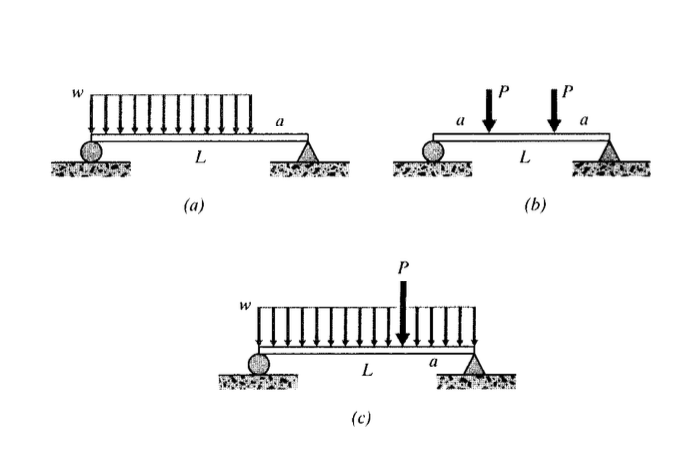
(a)-(h) Write expressions for the slope and deflection curves of the beams shown here.

Exercise \(\PageIndex{2}\)

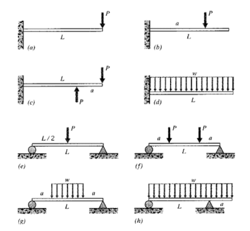
(a)-(h)Use MapleV (or other) software to plot the slope and deflection curves for the beams in Exercise \(\PageIndex{1}\), using the values (as needed) \(L = 25\ in, a = 15\ in, w = 10\ lb/in, P = 150\ lb\).

Exercise \(\PageIndex{3}\)

Show that the shape factor for shear for a circular cross section is

\(f_s = \dfrac{A}{I^2} \int_A \dfrac{Q}{b^2} dA = \dfrac{10}{9}\)

Exercise \(\PageIndex{4}\)

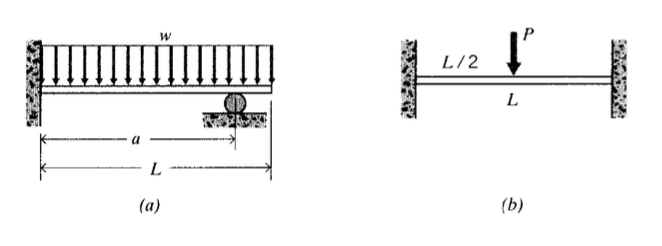
(a)-(b) Determine the deflection curves for the beams shown here. Plot these curves for the the values (as needed) \(L = 25\ in, a = 5\ in, w = 10\ lb/in, P = 150\ lb\).

Exercise \(\PageIndex{5}\)

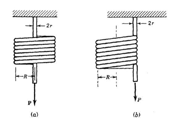
(a) Determine the deflection of a coil spring under the influence of an axial force \(F\), including the contribution of bending, direct shear, and torsional shear effects. Using \(r = 1\ mm\) and \(R = 10\ mm\), compute the relative magnitudes of the three contributions.

(b) Repeat the solution in (a), but take the axial load to be placed at the outer radius of the coil.

Exercise \(\PageIndex{6}\)

(a)-(c) Use the method of superposition to write expressions for the deflection curve \(\delta (x)\) for the cases shown here.