
4.2: Stresses in Beams
- Page ID
- 44541
\( \newcommand{\vecs}[1]{\overset { \scriptstyle \rightharpoonup} {\mathbf{#1}} } \)
\( \newcommand{\vecd}[1]{\overset{-\!-\!\rightharpoonup}{\vphantom{a}\smash {#1}}} \)
\( \newcommand{\dsum}{\displaystyle\sum\limits} \)
\( \newcommand{\dint}{\displaystyle\int\limits} \)
\( \newcommand{\dlim}{\displaystyle\lim\limits} \)
\( \newcommand{\id}{\mathrm{id}}\) \( \newcommand{\Span}{\mathrm{span}}\)
( \newcommand{\kernel}{\mathrm{null}\,}\) \( \newcommand{\range}{\mathrm{range}\,}\)
\( \newcommand{\RealPart}{\mathrm{Re}}\) \( \newcommand{\ImaginaryPart}{\mathrm{Im}}\)
\( \newcommand{\Argument}{\mathrm{Arg}}\) \( \newcommand{\norm}[1]{\| #1 \|}\)
\( \newcommand{\inner}[2]{\langle #1, #2 \rangle}\)
\( \newcommand{\Span}{\mathrm{span}}\)
\( \newcommand{\id}{\mathrm{id}}\)
\( \newcommand{\Span}{\mathrm{span}}\)
\( \newcommand{\kernel}{\mathrm{null}\,}\)
\( \newcommand{\range}{\mathrm{range}\,}\)
\( \newcommand{\RealPart}{\mathrm{Re}}\)
\( \newcommand{\ImaginaryPart}{\mathrm{Im}}\)
\( \newcommand{\Argument}{\mathrm{Arg}}\)
\( \newcommand{\norm}[1]{\| #1 \|}\)
\( \newcommand{\inner}[2]{\langle #1, #2 \rangle}\)
\( \newcommand{\Span}{\mathrm{span}}\) \( \newcommand{\AA}{\unicode[.8,0]{x212B}}\)
\( \newcommand{\vectorA}[1]{\vec{#1}} % arrow\)
\( \newcommand{\vectorAt}[1]{\vec{\text{#1}}} % arrow\)
\( \newcommand{\vectorB}[1]{\overset { \scriptstyle \rightharpoonup} {\mathbf{#1}} } \)
\( \newcommand{\vectorC}[1]{\textbf{#1}} \)
\( \newcommand{\vectorD}[1]{\overrightarrow{#1}} \)
\( \newcommand{\vectorDt}[1]{\overrightarrow{\text{#1}}} \)
\( \newcommand{\vectE}[1]{\overset{-\!-\!\rightharpoonup}{\vphantom{a}\smash{\mathbf {#1}}}} \)
\( \newcommand{\vecs}[1]{\overset { \scriptstyle \rightharpoonup} {\mathbf{#1}} } \)
\(\newcommand{\longvect}{\overrightarrow}\)
\( \newcommand{\vecd}[1]{\overset{-\!-\!\rightharpoonup}{\vphantom{a}\smash {#1}}} \)
\(\newcommand{\avec}{\mathbf a}\) \(\newcommand{\bvec}{\mathbf b}\) \(\newcommand{\cvec}{\mathbf c}\) \(\newcommand{\dvec}{\mathbf d}\) \(\newcommand{\dtil}{\widetilde{\mathbf d}}\) \(\newcommand{\evec}{\mathbf e}\) \(\newcommand{\fvec}{\mathbf f}\) \(\newcommand{\nvec}{\mathbf n}\) \(\newcommand{\pvec}{\mathbf p}\) \(\newcommand{\qvec}{\mathbf q}\) \(\newcommand{\svec}{\mathbf s}\) \(\newcommand{\tvec}{\mathbf t}\) \(\newcommand{\uvec}{\mathbf u}\) \(\newcommand{\vvec}{\mathbf v}\) \(\newcommand{\wvec}{\mathbf w}\) \(\newcommand{\xvec}{\mathbf x}\) \(\newcommand{\yvec}{\mathbf y}\) \(\newcommand{\zvec}{\mathbf z}\) \(\newcommand{\rvec}{\mathbf r}\) \(\newcommand{\mvec}{\mathbf m}\) \(\newcommand{\zerovec}{\mathbf 0}\) \(\newcommand{\onevec}{\mathbf 1}\) \(\newcommand{\real}{\mathbb R}\) \(\newcommand{\twovec}[2]{\left[\begin{array}{r}#1 \\ #2 \end{array}\right]}\) \(\newcommand{\ctwovec}[2]{\left[\begin{array}{c}#1 \\ #2 \end{array}\right]}\) \(\newcommand{\threevec}[3]{\left[\begin{array}{r}#1 \\ #2 \\ #3 \end{array}\right]}\) \(\newcommand{\cthreevec}[3]{\left[\begin{array}{c}#1 \\ #2 \\ #3 \end{array}\right]}\) \(\newcommand{\fourvec}[4]{\left[\begin{array}{r}#1 \\ #2 \\ #3 \\ #4 \end{array}\right]}\) \(\newcommand{\cfourvec}[4]{\left[\begin{array}{c}#1 \\ #2 \\ #3 \\ #4 \end{array}\right]}\) \(\newcommand{\fivevec}[5]{\left[\begin{array}{r}#1 \\ #2 \\ #3 \\ #4 \\ #5 \\ \end{array}\right]}\) \(\newcommand{\cfivevec}[5]{\left[\begin{array}{c}#1 \\ #2 \\ #3 \\ #4 \\ #5 \\ \end{array}\right]}\) \(\newcommand{\mattwo}[4]{\left[\begin{array}{rr}#1 \amp #2 \\ #3 \amp #4 \\ \end{array}\right]}\) \(\newcommand{\laspan}[1]{\text{Span}\{#1\}}\) \(\newcommand{\bcal}{\cal B}\) \(\newcommand{\ccal}{\cal C}\) \(\newcommand{\scal}{\cal S}\) \(\newcommand{\wcal}{\cal W}\) \(\newcommand{\ecal}{\cal E}\) \(\newcommand{\coords}[2]{\left\{#1\right\}_{#2}}\) \(\newcommand{\gray}[1]{\color{gray}{#1}}\) \(\newcommand{\lgray}[1]{\color{lightgray}{#1}}\) \(\newcommand{\rank}{\operatorname{rank}}\) \(\newcommand{\row}{\text{Row}}\) \(\newcommand{\col}{\text{Col}}\) \(\renewcommand{\row}{\text{Row}}\) \(\newcommand{\nul}{\text{Nul}}\) \(\newcommand{\var}{\text{Var}}\) \(\newcommand{\corr}{\text{corr}}\) \(\newcommand{\len}[1]{\left|#1\right|}\) \(\newcommand{\bbar}{\overline{\bvec}}\) \(\newcommand{\bhat}{\widehat{\bvec}}\) \(\newcommand{\bperp}{\bvec^\perp}\) \(\newcommand{\xhat}{\widehat{\xvec}}\) \(\newcommand{\vhat}{\widehat{\vvec}}\) \(\newcommand{\uhat}{\widehat{\uvec}}\) \(\newcommand{\what}{\widehat{\wvec}}\) \(\newcommand{\Sighat}{\widehat{\Sigma}}\) \(\newcommand{\lt}{<}\) \(\newcommand{\gt}{>}\) \(\newcommand{\amp}{&}\) \(\definecolor{fillinmathshade}{gray}{0.9}\)Introduction
Understanding of the stresses induced in beams by bending loads took many years to develop. Galileo worked on this problem, but the theory as we use it today is usually credited principally to the great mathematician Leonard Euler (1707–1783). As will be developed below, beams develop normal stresses in the lengthwise direction that vary from a maximum in tension at one surface, to zero at the beam’s midplane, to a maximum in compression at the opposite surface. Shear stresses are also induced, although these are often negligible in comparision with the normal stresses when the length-to-height ratio of the beam is large. The procedures for calculating these stresses for various loading conditions and beam cross-section shapes are perhaps the most important methods to be found in introductory Mechanics of Materials, and will be developed in the sections to follow. This theory requires that the user be able to construct shear and bending moment diagrams for the beam, as developed for instance in Module 12.
Normal Stresses
A beam subjected to a positive bending moment will tend to develop a concave-upward curvature. Intuitively, this means the material near the top of the beam is placed in compression along the \(x\) direction, with the lower region in tension. At the transition between the compressive and tensile regions, the stress becomes zero; this is the neutral axis of the beam. If the material tends to fail in tension, like chalk or glass, it will do so by crack initiation and growth from the lower tensile surface. If the material is strong in tension but weak in compression, it will fail at the top compressive surface; this might be observed in a piece of wood by a compressive buckling of the outer fibers.
We seek an expression relating the magnitudes of these axial normal stresses to the shear and bending moment within the beam, analogously to the shear stresses induced in a circular shaft by torsion. In fact, the development of the needed relations follows exactly the same direct approach as that used for torsion:
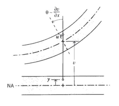
1. Geometrical statement: We begin by stating that originally transverse planes within the beam remain planar under bending, but rotate through an angle \(\theta\) about points on the neutral axis as shown in Figure 1. For small rotations, this angle is given approximately by the \(x\)-derivative of the beam's vertical deflection function \(v(x)\) (The exact expression for curvature is
\[\dfrac{d \theta}{ds} = \dfrac{d^2 v/dx^2}{[1 + (dv/dx)^2]^{3/2}}. \nonumber \]
This gives \(\theta \approx dv/dx\) when the squared derivative in the denominator is small compared to 1.):
\[u = -y v_{,x} \nonumber \]
where the comma indicates differentiation with respect to the indicated variable (\(v_{,x} \equiv dv/dx\)). Here \(y\) is measured positive upward from the neutral axis, whose location within the beam has not yet been determined.
2. Kinematic equation: The \(x\)-direction normal strain \(\epsilon_x\) is then the gradient of the displacement:
\[\epsilon_x = \dfrac{du}{dx} = -yv_{,xx} \nonumber \]
Note that the strains are zero at the neutral axis where \(y = 0\), negative (compressive) above the axis, and positive (tensile) below. They increase in magnitude linearly with \(y\), much as the shear strains increased linearly with \(r\) in a torsionally loaded circular shaft. The quantity \(v_{,xx} \equiv d^2v/dx^2\) is the spatial rate of change of the slope of the beam deflection curve, the "slope of the slope." This is called the curvature of the beam.
3. Constitutive equation: The stresses are obtained directly from Hooke’s law as
\[\sigma_x = E\epsilon_x = -y Ev_{,xx} \nonumber \]
This restricts the applicability of this derivation to linear elastic materials. Hence the axial normal stress, like the strain, increases linearly from zero at the neutral axis to a maximum at the outer surfaces of the beam.
4. Equilibrium relations: Since there are no axial (\(x\)-direction) loads applied externally to the beam, the total axial force generated by the normal \(\sigma_x\) stresses (shown in Figure 2) must be zero. This can be expressed as
\(\sum F_x = 0 = \int_A \sigma_x dA = \int_A -y Ev_{,xx} dA\)
which requires that
\(\int_A y dA = 0\)
The distance \(\bar{y}\) from the neutral axis to the centroid of the cross-sectional area is
\(\bar{y} = \dfrac{\int_A y dA}{\int_A dA}\)
Hence \(\bar{y} = 0\), i.e. the neutral axis is coincident with the centroid of the beam cross-sectional area. This result is obvious on reflection, since the stresses increase at the same linear rate, above the axis in compression and below the axis in tension. Only if the axis is exactly at the centroidal position will these stresses balance to give zero net horizontal force and keep the beam in horizontal equilibrium.
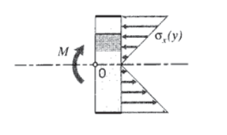
The normal stresses in compression and tension are balanced to give a zero net horizontal force, but they also produce a net clockwise moment. This moment must equal the value of \(M(x)\) at that value of \(x\), as seen by taking a moment balance around point \(O\):
\(\sum M_O = 0 = M + \int_A \sigma_x \cdot y dA\)
\[M = \int_A (y Ev_{,xx}) \cdot y dA = Ev_{,xx} \int_A y^2 dA \nonumber \]
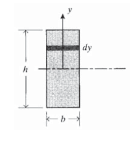
The quantity \(\int y^2 dA\) is the rectangular moment of inertia with respect to the centroidal axis, denoted \(I\). For a rectangular cross section of height \(h\) and width \(b\) as shown in Figure 3 this is:
\[I = \int_{-h/2}^{h/2} y^2 b dy = \dfrac{bh^3}{12} \nonumber \]
Solving Equation 4.2.4 for \(v_{,xx}\), the beam curvature is
\[v_{,xx} = \dfrac{M}{EI} \nonumber \]
5. An explicit formula for the stress can be obtained by using this in Equation 4.2.3:
\[\sigma_x = -y E \dfrac{M}{EI} = \dfrac{-My}{I} \nonumber \]
The final expression for stress, Equation 4.2.7, is similar to \(\tau_{\theta_z} = Tr/J\) for twisted circular shafts: the stress varies linearly from zero at the neutral axis to a maximum at the outer surface, it varies inversely with the moment of inertia of the cross section, and it is independent of the material’s properties. Just as a designer will favor annular drive shafts to maximize the polar moment of inertia \(J\), beams are often made with wide flanges at the upper and lower surfaces to increase \(I\).
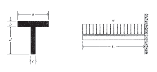
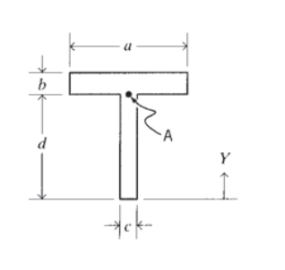
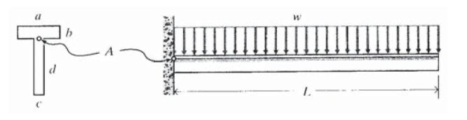
Consider a cantilevered T-beam with dimensions as shown in Figure 4, carrying a uniform loading of \(w N/m\). The maximum bending moment occurs at the wall, and is easily found to be \(M_{\max} = (wL)(L/2)\). The stress is then given by Equation 4.2.7, which requires that we know the location of the neutral axis (since \(y\) and \(I\) are measured from there).
The distance \(y\) from the bottom of the beam to the centroidal neutral axis can be found using the "composite area theorem" (see Exercise \(\PageIndex{1}\)). This theorem states that the distance from an arbitrary axis to the centroid of an area made up of several subareas is the sum of the subareas times the distance to their individual centroids, divided by the sum of the subareas( i.e. the total area):
\(\bar{y} = \dfrac{\sum_i A_i \bar{y}_i}{\sum_i A_i}\)
For our example, this is
\(\bar{y} = \dfrac{(d/2)(cd) + (d + b/2)(ab)}{cd + ab}\)
The moments of inertia of the individual parts of the compound area with respect to their own centroids are just \(ab^3/12\) and \(cd^3/12\). These moments can be referenced to the horizontal axis through the centroid of the compound area using the "parallel axis theorem" (see Exercise \(\PageIndex{3}\)). This theorem states that the moment of inertia \(I_{z'}\) of an area \(A\), relative to any arbitrary axis \(z'\) parallel to an axis through the centroid but a distance \(d\) from it, is the moment of inertia relative to the centroidal axis \(I_z\) plus the product of the area \(A\) and the square of the distance \(d\):
\(I_{z'} = I_z + A d^2\)
For our example, this is
The moment of inertia of the entire compound area, relative to its centroid, is then the sum of these two contributions:
\(I = I^{(1)} + I^{(2)}\)
The maximum stress is then given by Equation 4.2.7 using this value of \(I\) and \(y = \bar{y}/2\) (the distance from the neutral axis to the outer fibers), along with the maximum bending moment \(M_{\max}\). The result of these substitutions is
\(\sigma_x = \dfrac{(3d^2c + 6abd + 3ab^2)wL^2}{2c^2d^4 + 8abcd^3 + 12ab^2cd^2 + 8ab^3cd + 2a^2b^4}\)
In practice, each step would likely be reduced to a numerical value rather than working toward an algebraic solution.
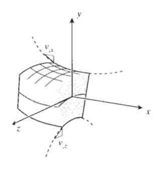
In pure bending (only bending moments applied, no transverse or longitudinal forces), the only stress is \(\sigma_x\) as given by Equation 4.2.7. All other stresses are zero (\(\sigma_y = \sigma_z = \tau_{xy} = \tau_{xz} = \tau_{yz} = 0\)). However, strains other than \(\epsilon_x\) are present, due to the Poisson effect. This does not generate shear strain \((\gamma_{xy} = \gamma_{xz} = \gamma_{yz} = 0)\), but the normal strains are
The strains can also be written in terms of curvatures. From Equation 4.2.2, the curvature along the beam is
\(v_{,xx} = -\dfrac{\epsilon_x}{y}\)
This is accompanied by a curvature transverse to the beam axis given by
\(v_{,zz} = -\dfrac{\epsilon_z}{y} = \dfrac{\nu\epsilon_x}{y} = -\nu v_{,xx}\)
This transverse curvature, shown in Figure 5, is known as anticlastic curvature; it can be seen by bending a "Pink Pearl" type eraser in the fingers.
As with tension and torsion structures, bending problems can often be done more easily with energy methods. Knowing the stress from Equation 4.2.7, the strain energy due to bending stress \(U_b\) can be found by integrating the strain energy per unit volume \(U^* = \sigma^2/2E\) over the specimen volume:
\(U_b = \int_V U^* dV = \int_L \int_A \dfrac{\sigma_x^2}{2E} dA dL\)
\(= \int_L \int_A \dfrac{1}{2E} (\dfrac{-My}{I})^2 dA dL = \int_L \dfrac{M^2}{2EI^2} \int_A y^2 dAdL\)
Since \(\int_A y^2 dA = I\), this becomes
\[U_b = \int_L \dfrac{M^2 dL}{2EI} \nonumber \]
If the bending moment is constant along the beam (definitely not the usual case), this becomes
\(U = \dfrac{M^2 L}{2EI}\)
This is another analog to the expression for uniaxial tension, \(U = P^2L/2AE\).
Buckling
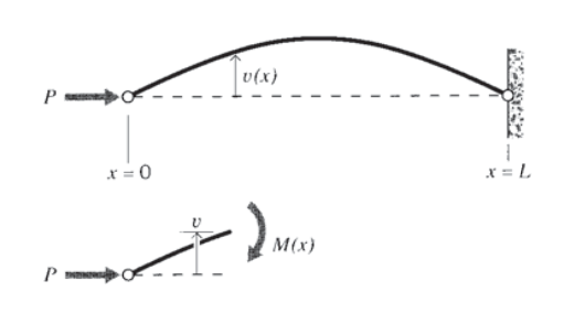
Long slender columns placed in compression are prone to fail by buckling, in which the column develops a kink somewhere along its length and quickly collapses unless the load is relaxed. This is actually a bending phenomenon, driven by the bending moment that develops if and when when the beam undergoes a transverse deflection. Consider a beam loaded in axial compression and pinned at both ends as shown in Figure 6. Now let the beam be made to deflect transversely by an amount v, perhaps by an adventitious sideward load or even an irregularity in the beam’s cross section. Positions along the beam will experience a moment given by
\[M(x) = Pv(x) \nonumber \]
The beam's own stiffness will act to restore the deflection and recover a straight shape, but the effect of the bending moment is to deflect the beam more. It’s a battle over which influence wins out. If the tendency of the bending moment to increase the deflection dominates over the ability of the beam’s elastic stiffness to resist bending, the beam will become unstable, continuing to bend at an accelerating rate until it fails.
The bending moment is related to the beam curvature by Equation 4.2.6, so combining this with Equation 4.2.9 gives
\[v_{,xx} = \dfrac{P}{EI} v \nonumber \]
Of course, this governing equation is satisfied identically if \(v = 0\), i.e. the beam is straight. We wish to look beyond this trivial solution, and ask if the beam could adopt a bent shape that would also satisfy the governing equation; this would imply that the stiffness is insufficient to restore the unbent shape, so that the beam is beginning to buckle. Equation 4.2.10 will be satisfied by functions that are proportional to their own second derivatives. Trigonometric functions have this property, so candidate solutions will be of the form
\(v = c_1 \sin \sqrt{\dfrac{P}{EI}} x + c_2 \cos \sqrt{\dfrac{P}{EI}} x\)
It is obvious that \(c_2\) must be zero, since the deflection must go to zero at \(x = 0\) and \(L\). Further, the sine term must go to zero at these two positions as well, which requires that the length \(L\) be exactly equal to a multiple of the half wavelength of the sine function:
\(\sqrt{\dfrac{P}{EI} L} = n\pi, n = 1, 2, 3, \cdots\)
The lowest value of \(P\) leading to the deformed shape corresponds to \(n = 1\); the critical buckling load \(P_{cr}\) is then:
\[P_{cr} = \dfrac{\pi^2 EI}{L^2} \nonumber \]
Note the dependency on \(L^2\), so the buckling load drops with the square of the length.
This strong dependency on length shows why crossbracing is so important in preventing buckling. If a brace is added at the beam’s midpoint as shown in Figure 7 to eliminate deflection there, the buckling shape is forced to adopt a wavelength of \(L\) rather than 2\(L\). This is equivalent to making the beam half as long, which increases the critical buckling load by a factor of four.
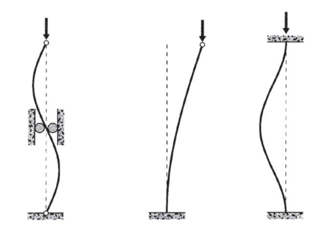
Similar reasoning can be used to assess the result of having different support conditions. If for instance the beam is cantilevered at one end but unsupported at the other, its buckling shape will be a quarter sine wave. This is equivalent to making the beam twice as long as the case with both ends pinned, so the buckling load will go down by a factor of four. Cantilevering both ends forces a full-wave shape, with the same buckling load as the pinned beam with a midpoint support.
Shear stresses
Transverse loads bend beams by inducing axial tensile and compressive normal strains in the beam's \(x\)-direction, as discussed above. In addition, they cause shear effects that tend to slide vertical planes tangentially to one another as depicted in Figure 8, much like sliding playing cards past one another. The stresses \(\tau_{xy}\) associated with this shearing effect add up to the vertical shear force we have been calling \(V\), and we now seek to understand how these stresses are distributed over the beam's cross section. The shear stress on vertical planes must be accompanied by an equal stress on horizontal planes since \(\tau_{xy} = \tau_{yx}\), and these horizontal shearing stresses must become zero at the upper and lower surfaces of the beam unless a traction is applied there to balance them. Hence they must reach a maximum somewhere within the beam.
The variation of this horizontal shear stress with vertical position y can be determined by examining a free body of width \(dx\) cut from the beam a distance y above neutral axis as shown in Figure 9. The moment on the left vertical face is \(M(x)\), and on the right face it has increased to \(M + dM\). Since the horizontal normal stresses are directly proportional to the moment (\(\sigma x = My/I\)), any increment in moment dM over the distance \(dx\) produces an imbalance in the horizontal force arising from the normal stresses. This imbalance must be compensated by a shear stress \(\tau_{xy}\) on the horizontal plane at \(y\). The horizontal force balance is written as
\(\tau_{xy} b dx = \int_{A'} \dfrac{dM \xi}{I} dA'\)
Figure 8: Shearing displacements in beam bending.
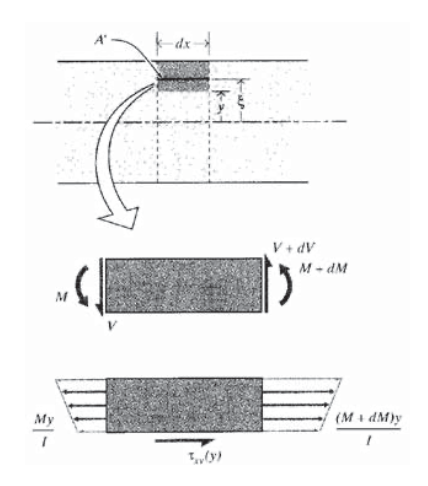
Figure 9: Shear and bending moment in a differential length of beam.
where \(b\) is the width of the beam at \(y, \xi\) is a dummy height variable ranging from \(y\) to the outer surface of the beam, and \(A'\) is the cross-sectional area between the plane at \(y\) and the outer surface. Using \(dM = V\ dx\) from Equation 4.2.8 of Module 12, this becomes
\[\tau_{xy} = \dfrac{V}{Ib} \int_A' \xi dA' = \dfrac{VQ}{Ib} \nonumber \]
where here \(Q(y) = \int_{A'} \xi dA' = \bar{\xi} A'\) is the first moment of the area above \(y\) about the neutral axis.
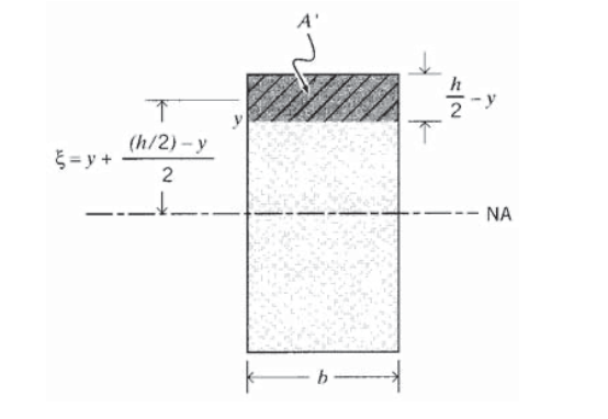
The parameter \(Q(y)\) is notorious for confusing persons new to beam theory. To determine it for a given height \(y\) relative to the neutral axis, begin by sketching the beam cross section, and draw a horizontal line line at the position \(y\) at which \(Q\) is sought (Figure 10 shows a rectangular beam of of constant width \(b\) and height \(h\) for illustration). Note the area \(A'\) between this line and the outer surface (indicated by cross-hatching in Figure 10). Now compute the distance \(\bar{\xi}\) from the neutral axis to the centroid of \(A'\). The parameter \(Q(y)\) is the product of \(A'\) and \(\xi\); this is the first moment of the area \(A'\) with respect to the centroidal axis. For the rectangular beam, it is
Note that \(Q(y)\), and therefore \(\tau_{xy}(y)\) as well, is parabolic, being maximum at the neutral axis (\(y\) = 0) and zero at the outer surface (\(y = h/2\)). Using \(I = bh^3/12\) for the rectangular beam, the maximum shear stress as given by Equation 4.2.12 is
\(\tau_{xy, \max} = \tau_{xy}|_{y = 0} = \dfrac{3V}{2bh}\)
(Keep in mind than the above two expressions for \(Q\) and \(\tau_{xy,\max}\) are for rectangular cross section only; sections of other shapes will have different results.) These shear stresses are most important in beams that are short relative to their height, since the bending moment usually increases with length and the shear force does not (see Exercise \(\PageIndex{11}\)). One standard test for interlaminar shear strength("Apparent Horizontal Shear Strength of Reinforced Plastics by Short Beam Method," ASTM D2344, American Society for Testing and Materials.) is to place a short beam in bending and observe the load at which cracks develop along the midplane.
Since the normal stress is maximum where the horizontal shear stress is zero (at the outer fibers), and the shear stress is maximum where the normal stress is zero (at the neutral axis), it is often possible to consider them one at a time. However, the juncture of the web and the flange in I and T beams is often a location of special interest, since here both stresses can take on substantial values.
Consider the T beam seen previously in Example \(\PageIndex{1}\), and examine the location at point \(A\) shown in Figure 11, in the web immediately below the flange. Here the width \(b\) in Equation 4.2.12 is the dimension labeled \(c\); since the beam is thin here the shear stress \(\tau_{xy}\) will tend to be large, but it will drop dramatically in the flange as the width jumps to the larger value a. The normal stress at point \(A\) is computed from \(\sigma_x = My/I\), using \(y = d − y\). This value will be almost as large as the outer-fiber stress if the flange thickness b is small compared with the web height \(d\). The Mohr’s circle for the stress state at point \(A\) would then have appreciable contributions from both \(\sigma_x\) and \(\tau_{xy}\), and can result in a principal stress larger than at either the outer fibers or the neutral axis.
This problem provides a good review of the governing relations for normal and shear stresses in beams, and is also a natural application for symbolic-manipulation computer methods. Using Maple software, we might begin by computing the location of the centroidal axis:
Here the ">" symbol is the Maple prompt, and the ";" is needed by Maple to end the command. The maximum shear force and bending moment (present at the wall) are defined in terms of the distributed load and the beam length as
> ybar := ((d/2)*c*d) + ( (d+(b/2) )*a*b )/( c*d + a*b );
For plotting purposes, it will be convenient to have a height variable Y measured from the bottom of the section. The relations for normal stress, shear stress, and the first principal stress are functions of Y; these are defined using the Maple “procedure” command:
> V := w*L;
> M := -(w*L)*(L/2);
For plotting purposes, it will be convenient to have a height variable Y measured from the bottom of the section. The relations for normal stress, shear stress, and the first principal stress are functions of Y; these are defined using the Maple “procedure” command:
> sigx := proc (Y) -M*(Y-ybar)/Iz end;
> tauxy := proc (Y) V*Q(Y)/(Iz*B(Y) ) end;
> sigp1 := proc (Y) (sigx(Y)/2) + sqrt( (sigx(Y)/2)^2 + (tauxy(Y))^2 ) end;
The moment of inertia Iz is computed as
> I1 := (a*b^3)/12 + a*b* (d+(b/2)-ybar)^2;
> I2 := (c*d^3)/12 + c*d* ((d/2)-ybar)^2;
> Iz := I1+I2;
The beam width B is defined to take the appropriate value depending on whether the variable Y is in the web or the flange:
> B:= proc (Y) if Y<d then B:=c else B:=a fi end;
The command "fi" ("if" spelled backwards) is used to end an if-then loop. The function Q(Y) is defined for the web and the flange separately:
> Q:= proc (Y) if Y<d then
>      int( (yy-ybar)*c,yy=Y..d) + int( (yy-ybar)*a,yy=d..(d+b) )
>    else
>      int( (yy-ybar)*a,yy=Y.. (d+b) )
>    fi end;
Here "int" is the Maple command for integration, and yy is used as the dummy height variable. The numerical values of the various parameters are defined as
> a:=3: b:=1/4: c:=1/4: d:=3-b: L:=8: w:=100:
Finally, the stresses can be graphed using the Maple plot command
> plot({sigx,tauxy,sigp1},Y=0..3,sigx=-500..2500);
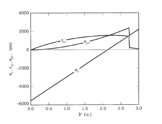
The resulting plot is shown in Figure 12.
In the previous example, we were interested in the variation of stress as a function of height in a beam of irregular cross section. Another common design or analysis problem is that of the variation of stress not only as a function of height but also of distance along the span dimension of the beam. The shear and bending moments \(V(x)\) and \(M(x)\) vary along this dimension, and so naturally do the stresses \(\sigma_x (x,y)\) and \(\tau_{xy} (x,y)\) that depend on them according to Equation 4.2.7 and 4.2.12.
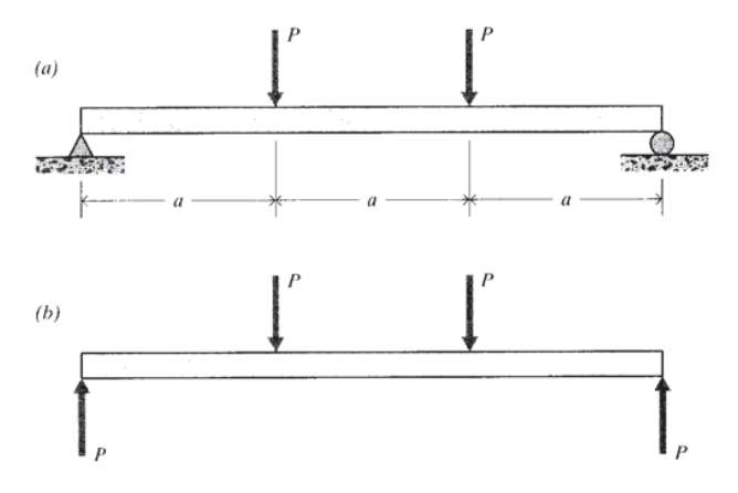
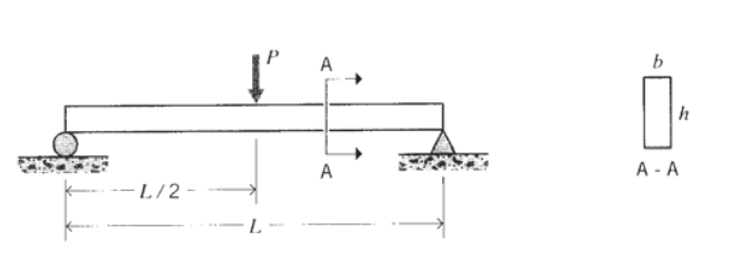
Consider a short beam of rectangular cross section subjected to four-point loading as seen in Figure 13. The loading, shear, and bending moment functions are:
The shear and normal stresses can be determined as functions of \(x\) and \(y\) directly from these functions, as well as such parameters as the principal stress. Since \(\sigma_y\) is zero everywhere, the principal stress is
\(\sigma_{p1} = \dfrac{\sigma_x}{2} + \sqrt{(\dfrac{\sigma_x}{2})^2 + \tau_{xy}^2}\)
One way to visualize the x-y variation of \(\sigma_{p1}\) is by means of a 3D surface plot, which can be prepared easily by Maple. For the numerical values \(P = 100, a = h = 10, b = 3\), we could use the expressions (Maple responses removed for brevity):
> # use Heaviside for singularity functions
> readlib(Heaviside);
> sfn := proc(x,a,n) (x-a)^n * Heaviside(x-a) end;
> # define shear and bending moment functions
> V:=(x)-> -P*sfn(x,0,0)+P*sfn(x,a,0)+P*sfn(x,2*a,0)-P*sfn(x,3*a,0);
> M:=(x)-> P*sfn(x,0,1)-P*sfn(x,a,1)-P*sfn(x,2*a,1)+P*sfn(x,3*a,1);
> # define shear stress function
> tau:=V(x)*Q/(Iz*b);
> Q:=(b/2)*( (h^2/4) -y^2);
> Iz:=b*h^3/12;
> # define normal stress function
> sig:=M(x)*y/Iz;
> # define principal stress
> sigp:= (sig/2) + sqrt( (sig/2)^2 + tau^2 );
> # define numerical parameters
> P:=100;a:=10;h:=10;b:=3;
> # make plot
> plot3d(sigp,x=0..3*a,y=-h/2 .. h/2);
The resulting plot is shown in Figure 14. The dominance of the parabolic shear stress is evident near the beam ends, since here the shear force is at its maximum value but the bending moment is small (plot the shear and bending moment diagrams to confirm this). In the central part of the beam, where \(a < x < 2a\), the shear force vanishes and the principal stress is governed only by the normal stress \(\sigma_x\), which varies linearly from the beam’s neutral axis. The first principal stress is zero in the compressive lower part of this section, since here the normal stress \(\sigma_x\) is negative and the right edge of the Mohr’s circle must pass through the zero value of the other normal stress \(\sigma_y\). Working through the plot of Figure 14 is a good review of the beam stress formulas.
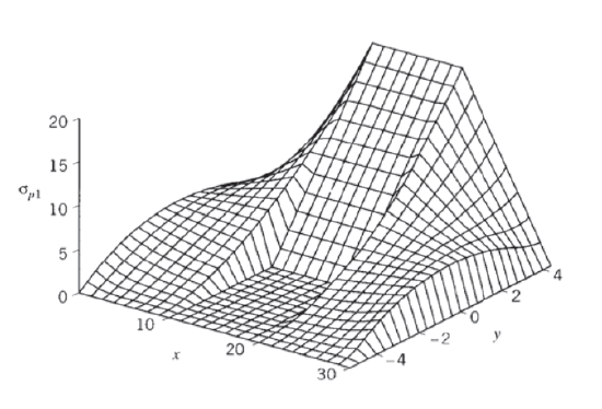
Figure 14: Variation of principal stress \(\sigma_{p1}\) in four-point bending.
Derive the composite area theorem for determining the centroid of a compound area.
\(\bar{y} = \dfrac{\sum_i A_i \bar{y}_i}{\sum_i A_i}\)
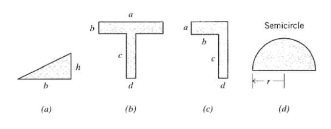
(a)-(d) Locate the centroids of the areas shown.
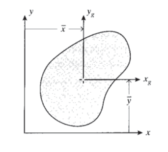
Derive the "parallel-axis theorem" for moments of inertia of a plane area:
\(I_x = I_{xg} + A \bar{y}^2\)
\(I_y = I_{yg} + A \bar{x}^2\)
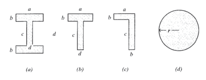
(a)-(d) Determine the moment of inertia relative to the horizontal centroidal axis of the areas shown.
Show that the moment of inertia transforms with respect to axis rotations exactly as does the stress:
where \(I_x\) and \(I_y\) are the moments of inertia relative to the \(x\) and \(y\) axes respectively and \(I_{xy}\) is the product of inertia defined as
\(I_{xy} = \int_A xy dA\)
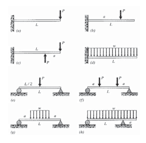
(a)–(h) Determine the maxiumum normal stress σx in the beams shown here, using the values (as needed) \(L = 25\ in\), \(a = 5 \ in\), \(w = 10\ lb/in\), \(P = 150\ lb\). Assume a rectangular cross-section of width \(b = 1\) in and height \(h = 2\ in\).
Justify the statement in ASTM test D790, "Standard Test Methods for Flexural Properties of Unreinforced and Reinforced Plastics and Electrical Insulating Materials," which reads:
When a beam of homogeneous, elastic material is tested in flexure as a simple beam supported at two points and loaded at the midpoint, the maximum stress in the outer fibers occurs at midspan. This stress may be calculated for any point on the load-deflection curve by the following equation:
\(S = 3PL/2bd^2\)
where \(S\) = stress in the outer fibers at midspan, MPa; \(P\) = load at a given point on the load-deflection curve; \(L\) = support span, mm; \(b\) = width of beam tested, mm; and d = depth of beam tested, mm.
Justify the statement in ASTM test D790, "Standard Test Methods for Flexural Properties of Unreinforced and Reinforced Plastics and Electrical Insulating Materials," which reads:
The tangent modulus of elasticity, often called the "modulus of elasticity," is the ratio, within the elastic limit of stress to corresponding strain and shall be expressed in megapascals. It is calculated by drawing a tangent to the steepest initial straight-line portion of the load-deflection curve and using [the expression:]
\(E_b = L^3 m/4bd^3\)
where \(E_b\) = modulus of elasticity in bending, MPa; \(L\) = support span, mm; \(d\) = depth of beam tested, mm; and \(m\) = slope of the tangent to the initial straight-line portion of the load-deflection curve, \(N/mm\) of deflection.
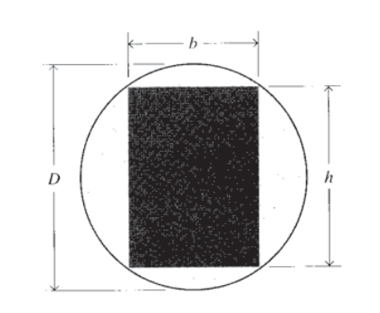
A rectangular beam is to be milled from circular stock as shown. What should be the ratio of height to width \((b/h)\) to as to minimize the stresses when the beam is put into bending?
(a)-(h) Determine the maxiumum shear τxy in the beams of Exercise \(\PageIndex{6}\), , using the values (as needed) \(L = 25\ in, a = 5\ in, w = 10\ lb/in, P = 150\ lb\). Assume a rectangular cross-section of width \(b = 1\) in and height \(h = 2\ in\).
Show that the ratio of maximum shearing stress to maximum normal stress in a beam subjected to 3-point bending is
\(\dfrac{\tau}{\sigma} = \dfrac{h}{2L}\)
Hence the importance of shear stress increases as the beam becomes shorter in comparison with its height.
Read the ASTM test D4475, "Standard Test Method for Apparent Horizontal Shear Strength of Pultruded Reinforced Plastic Rods By The Short-Beam Method," and justify the expression given there for the apparent shear strength:
\(S = 0.849 P/d^2\)
where \(S\) = apparent shear strength, \(N/m^2\), (or psi); \(P\) = breaking load, \(N\), (or lbf); and \(d\) = diameter of specimen, m (or in.).
For the T beam shown here, with dimensions \(L = 3, a = 0.05, b = 0.005, c = 0.005, d = 0.7\) (all in \(m\)) and a loading distribution of \(w = 5000 N/m\), determine the principal and maximum shearing stress at point \(A\).
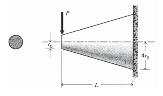
Determine the maximum normal stress in a cantilevered beam of circular cross section whose radius varies linearly from \(4r_0\) to \(r_0\) in a distance \(L\), loaded with a force \(P\) at the free end.
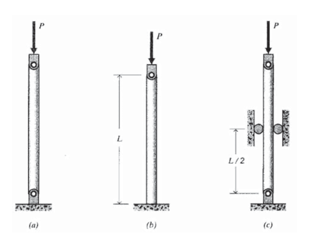
A carbon steel column has a length \(L = 1\ m\) and a circular cross section of diameter \(d = 20\ mm\). Determine the critical buckling load \(P_c\) for the case of (a) both ends pinned, (b) one end cantilevered, (c) both ends pinned but supported laterally at the midpoint.
A carbon steel column has a length \(L = 1\ m\) and a circular cross section. Determine the diameter \(d\) at which the column has an equal probablity of buckling or yielding in compression.