4.4: Laminated Composite Plates

Introduction

This document is intended to outline the mechanics of fiber-reinforced laminated plates, leading to a computational scheme that relates the in-plane strain and curvature of a laminate to the tractions and bending moments imposed on it. Although this is a small part of the overall field of fiber-reinforced composites, or even of laminate theory, it is an important technique that should be understood by all composites engineers.

In the sections to follow, we will review the constitutive relations for isotropic materials in matrix form, then show that the extension to transversely isotropic composite laminae is very straightforward. Since each ply in a laminate may be oriented arbitrarily, we will then show how the elastic properties of the individual laminae can be transformed to a common direction. Finally, we will balance the individual ply stresses against the applied tractions and moments to develop matrix governing relations for the laminate as a whole.

The calculations for laminate mechanics are best done by computer, and algorithms are outlined for elastic laminates, laminates exhibiting thermal expansion effects, and laminates exhibiting viscoelastic response.

Isotropic linear elastic materials

As shown in elementary texts on Mechanics of Materials (cf. Roylance 1996(See References listed at the end of this document.)), the Cartesian strains resulting from a state of plane stress (\(\sigma_z = \tau_{xz} = \tau_{yz} = 0\)) are

\(\gamma_{xy} = \dfrac{1}{G} \tau_{xy}\)

In plane stress there is also a strain in the \(z\) direction due to the Poisson effect: \(\epsilon_z = -\nu (\sigma_x + \sigma_y)\); this strain component will be ignored in the sections to follow. In the above relations there are three elastic constants: the Young's modulus \(E\), Poisson's ratio \(\nu\), and the shear modulus \(G\). However, for isotropic materials there are only two independent elastic constants, and for instance \(G\) can be obtained from \(E\) and \(\nu\) as

\(G = \dfrac{E}{2(1 + \nu)}\)

Using matrix notation, these relations can be written as

\[\left \{ \begin{array} {c} {\epsilon_x} \\ {\epsilon_x} \\ {\gamma_{xy}} \end{array} \right \} = \begin{bmatrix} 1/E & -\nu/E & 0 \\ -\nu/E & 1/E & 0 \\ 0 & 0 & 1/G \end{bmatrix} \left \{ \begin{array} {c} {\sigma_x} \\ {\sigma_y} \\ {\tau_{xy}} \end{array} \right \}\]

The quantity in brackets is called the compliance matrix of the material, denoted \(S\) or \(S_{ij}\). It is important to grasp the physical significance of its various terms. Directly from the rules of matrix multiplication, the element in the \(i^{th}\) row and \(j^{th}\) column of \(S_{ij}\) is the contribution of the \(j^{th}\) stress to the \(i^{th}\) strain. For instance the component in the 1,2 position is the contribution of the \(y\)-direction stress to the \(x\)-direction strain: multiplying \(\sigma_y\) by \(1/E\) gives the \(y\)-direction strain generated by \(\sigma_y\), and then multiplying this by \(-\nu\) gives the Poisson strain induced in the \(x\) direction. The zero elements show the lack of coupling between the normal and shearing components.

If we wish to write the stresses in terms of the strains, Equation 4.4.1 can be inverted to give:

\[\left \{ \begin{array} {c} {\sigma_x} \\ {\sigma_y} \\ {\tau_{xy}} \end{array} \right \} = \dfrac{E}{1- \nu^2} \begin{bmatrix} 1 & \nu & 0 \\ \nu & 1 & 0 \\ 0 & 0 & (1 - \nu)/2 \end{bmatrix} \left \{ \begin{array} {c} {\epsilon_x} \\ {\epsilon_y} \\ {\gamma_{xy}} \end{array} \right \}\]

where here \(G\) has been replaced by \(E/2(1 + \nu)\). This relation can be abbreviated further as:

\[\sigma = D \epsilon\]

where \(D = S^{-1}\) is the stiffness matrix. Note that the Young's modulus can be recovered by taking the reciprocal of the 1,1 element of the compliance matrix \(S\), but that the 1,1 position of the stiffness matrix \(D\) contains Poisson effects and is not equal to \(E\).

Anisotropic Materials

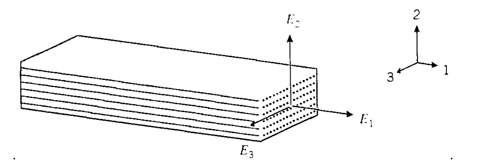
If the material has a texture like wood or unidirectionally-reinforced fiber composites as shown in Figure 1, the modulus \(E_1\) in the fiber direction will typically be larger than those in the transverse directions (\(E_2\) and \(E_3\)). When \(E_1 \ne E_2 \ne E_3\), the material is said to be orthotropic. It is common, however, for the properties in the plane transverse to the fiber direction to be isotropic to a good approximation (\(E_2 = E_3\)); such a material is called transversely isotropic. The elastic constitutive laws must be modified to account for this anisotropy, and the following form is an extension of the usual equations of isotropic elasticity to transversely isotropic materials:

\[\left \{ \begin{array} {c} {\epsilon_1} \\ {\epsilon_2} \\ {\gamma_{12}} \end{array} \right \} = \begin{bmatrix} 1/E_1 & -\nu_{21}/E_2 & 0 \\ -\nu_{12}/E_1 & 1/E_2 & 0 \\ 0 & 0 & 1/G_{12} \end{bmatrix} \left \{ \begin{array} {c} {\sigma_1} \\ {\sigma_2} \\ {\tau_{12}} \end{array} \right \}\]

Figure 1: An orthotropic material.

The parameter \(\nu_{12}\) is the principal Poisson's ratio; it is the ratio of the strain induced in the 2-direction by a strain applied in the 1-direction. This parameter is not limited to values less than 0.5 as in isotropic materials. Conversely, \(\nu_{21}\) gives the strain induced in the 1-direction by a strain applied in the 2-direction. Since the 2-direction (transverse to the fibers) usually has much less stiffness than the 1-direction, a given strain in the 1-direction will usually develop a much larger strain in the 2-direction than will the same strain in the 2-direction induce a strain in the 1-direction. Hence we will usually have \(\nu_{12} > \nu_{21}\). There are five constants in the above equation (\(E_1, E_2, \nu_{12}, \nu_{21}\) and \(G_{12}\). However, only four of them are independent; since the \(S\) matrix is symmetric, we have \(\nu_{21}/E_2 = \nu_{12}/E_1\).

The simple form of Equation 4.4.4, with zeroes in the terms representing coupling between normal and shearing components, is obtained only when the axes are aligned along the principal material directions; i.e. along and transverse to the fiber axes. If the axes are oriented along some other direction, all terms of the compliance matrix will be populated, and the symmetry of the material will not be evident. If for instance the fiber direction is off-axis from the loading direction, the material will develop shear strain as the fibers try to orient along the loading direction. There will therefore be a coupling between a normal stress and a shearing strain, which does not occur in an isotropic material.

Transformation of Axes

It is important to be able to transform the axes to and from the "laboratory" \(x - y\) frame to a natural material frame in which the axes might be labeled 1 - 2 corresponding to the fiber and transverse directions as shown in Figure 2.

Figure 2: Rotation of axes.

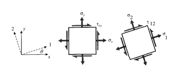
As shown in elementary textbooks, the transformation law for Cartesian Cauchy stress can be written:

\[\begin{array} {rcl} {\sigma_1} & = & {\sigma_x \cos^2 \theta + \sigma_y \sin^2 \theta + 2 \tau_{xy} \sin \theta \cos \theta} \\ {\sigma_2} & = & {\sigma_x \sin^2 \theta + \sigma_y \cos^2 \theta - 2 \tau_{xy} \sin \theta \cos \theta} \\ {\tau_{12}} & = & {(\sigma_y - \sigma_x) \sin \theta \cos \theta + \tau_{xy} (\cos^2 \theta -\sin^2 \theta)} \end{array}\]

Where \(\theta\) is the angle from the \(x\) axis to the 1 (fiber) axis. These relations can be written in matrix form as

\[\left \{ \begin{array} {c} {\sigma_1} \\ {\sigma_2} \\ {\tau_{12}} \end{array} \right \} = \dfrac{E}{1- \nu^2} \begin{bmatrix} c^2 & s^2 & 2sc \\ s^2 & c^2 & -2sc \\ -sc & sc & c^2 - s^2 \end{bmatrix} \left \{ \begin{array} {c} {\sigma_x} \\ {\sigma_y} \\ {\tau_{xy}} \end{array} \right \}\]

where \(c = \cos \theta\) and \(s = \sin \theta\). This can be abbreviated as

\[\sigma' = A \sigma\]

where \(A\) is the transformation matrix in brackets above. This expression could be applied to three-dimensional as well as two-dimensional stress states, although the particular form of \(A\) given in Equation 4.4.6 is valid in two dimensions only (plane stress), and for Cartesian coordinates.

Using either mathematical or geometric arguments, it can be shown that the components of infinitesimal strain transform by almost the same relations:

\[\left \{ \begin{array} {c} {\epsilon_1} \\ {\epsilon_2} \\ {\tfrac{1}{2} \gamma_{12}} \end{array} \right \} = A \left \{ \begin{array} {c} {\epsilon_x} \\ {\epsilon_y} \\ {\tfrac{1}{2} \gamma_{xy}} \end{array} \right \} \]

The factor of 1/2 on the shear components arises from the classical definition of shear strain, which is twice the tensorial shear strain. This introduces some awkwardness into the transformation relations, which can be reduced by introducing the Reuter's matrix, defined as

\[[R] = \begin{bmatrix} 1 & 0 & 0 \\ 0 & 1 & 0 \\ 0 & 0 & 2 \end{bmatrix} \ \ or \ \ [R]^{-1} = \begin{bmatrix} 1 & 0 & 0 \\ 0 & 1 & 0 \\ 0 & 0 & \tfrac{1}{2} \end{bmatrix}\]

We can now write:

\(\left \{ \begin{array} {c} {\epsilon_1} \\ {\epsilon_2} \\ { \gamma_{12}} \end{array} \right \} = R \left \{ \begin{array} {c} {\epsilon_1} \\ {\epsilon_2} \\ {\tfrac{1}{2} \gamma_{12}} \end{array} \right \} = RA \left \{ \begin{array} {c} {\epsilon_x} \\ {\epsilon_y} \\ {\tfrac{1}{2} \gamma_{xy}} \end{array} \right \} = RAR^{-1} \left \{ \begin{array} {c} {\epsilon_x} \\ {\epsilon_y} \\ {\gamma_{xy}} \end{array} \right \}\)

or

\[\epsilon' = RAR^{-1} \epsilon\]

The transformation law for compliance can now be developed from the transformation laws for strains and stresses. By successive transformations, the strain in an arbitrary \(x-y\) direction is related to strain in the 1-2 (principal material) directions, then to the stresses in the 1-2 directions, and finally to the stresses in the \(x-y\) directions. The final grouping of transformation matrices relating the \(x-y\) strains to the \(x-y\) stresses is then the transformed compliance matrix in the \(x-y\) direction:

\(\left \{ \begin{array} {c} {\epsilon_x} \\ {\epsilon_y} \\ { \gamma_{xy}} \end{array} \right \} = R \left \{ \begin{array} {c} {\epsilon_x} \\ {\epsilon_y} \\ {\tfrac{1}{2} \gamma_{xy}} \end{array} \right \} = RA^{-1} \left \{ \begin{array} {c} {\epsilon_1} \\ {\epsilon_2} \\ {\tfrac{1}{2} \gamma_{12}} \end{array} \right \} = RA^{-1} R^{-1} \left \{ \begin{array} {c} {\epsilon_1} \\ {\epsilon_2} \\ { \gamma_{12}} \end{array} \right \}\)

\(=RA^{-1} R^{-1} S \left \{ \begin{array} {c} {\sigma_1} \\ {\sigma_2} \\ { \tau_{12}} \end{array} \right \} = RA^{-1} R^{-1} SA \left \{ \begin{array} {c} {\sigma_x} \\ {\sigma_y} \\ { \tau_{xy}} \end{array} \right \} \equiv \bar{S} \left \{ \begin{array} {c} {\sigma_x} \\ {\sigma_y} \\ { \tau_{xy}} \end{array} \right \}\)

where \(\bar{S}\) is the transformed compliance matrix relative to \(x-y\) axes. The inverse of \(\bar{S}\) is \(\bar{D}\), the stiffness matrix relative to \(x-y\) axes:

\[\bar{S} = RA^{-1} R^{-1} SA, \ \ \bar{D} = \bar{S}^{-1}\]

Example \(\PageIndex{1}\)

Consider a ply of Kevlar-epoxy composite with a stiffnesses \(E_1 = 82, E_2 = 4, G_{12} = 2.8\) (all GPa) and \(\nu_{12} = 0.25\). oriented at \(30^{\circ}\) from the \(x\) axis. The stiffness in the \(x\) direction can be found as the reciprocal of the 1,1 element of the transformed compliance matrix \(S\), as given by Equation 4.4.11. The following shows how this can be done with Maple symbolic mathematics software (edited for brevity):

Read linear algebra package
> with(linalg):
Define compliance matrix
> S:=matrix(3,3,[[1/E[1],-nu[21]/E[2],0],[-nu[12]/E[1],1/E[2],0],[0,0,1/G[12]]]); 
Numerical parameters for Kevlar-epoxy
> Digits:=4;unprotect(E);E[1]:=82e9;E[2]:=4e9;G[12]:=2.8e9;nu[12]:=.25; 
nu[21]:=nu[12]*E[2]/E[1];
Compliance matrix evaluated
> S2:=map(eval,S); 

\(S2 := \begin{bmatrix} .122010^{-10} & -.305010^{-11} & 0 \\ -.304910^{-11} & .250010^{-9} & 0 \\ 0 & 0 & .357110^{-9} \end{bmatrix} \)

Transformation matrix
> A:=matrix(3,3,[[c^2,s^2,2*s*c],[s^2,c^2,-2*s*c],[-s*c,s*c,c^2-s^2]]); 
Trigonometric relations and angle
> s:=sin(theta);c:=cos(theta);theta:=30*Pi/180;
Transformation matrix evaluated
> A2:=evalf(map(eval,A)); 

\(A2 := \begin{bmatrix} .7500 & .2500 & .8660 \\ .2500 & .7500 & -.8660 \\ -.4330 & .4330 & .5000 \end{bmatrix} \)

Reuter's matrix
> R:=matrix(3,3,[[1,0,0],[0,1,0],[0,0,2]]);
Transformed compliance matrix
> Sbar:=evalf(evalm( R &* inverse(A2) &* inverse(R) &* S2 &* A2 )); 

\(Sbar := \begin{bmatrix} .882810^{-10} & -.196810^{-10} & -.122210^{-9} \\ -.196910^{-10} & .207110^{-9} & -.837010^{-10} \\ -.122210^{-9} & -.837710^{-10} & .290510^{-9} \end{bmatrix} \)

Stiffness in x-direction
> 'E[x]'=1/Sbar[1,1]; 

\(E_x = .113310^{11}\)

Note that the transformed compliance matrix is symmetric (to within numerical roundoff error), but that nonzero coupling values exist. A user not aware of the internal composition of the material would consider it completely anisotropic.

Laminated composite plates

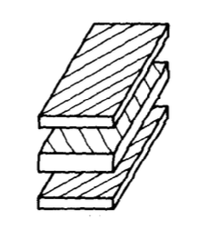
One of the most common forms of fiber-reinforced composite materials is the crossplied laminate, in which the fabricator "lays up" a sequence of unidirectionally reinforced "plies" as indicated in Figure 3. Each ply is typically a thin (approximately 0.2 mm) sheet of collimated fibers impregnated with an uncured epoxy or other thermosetting polymer matrix material. The orientation of each ply is arbitrary, and the layup sequence is tailored to achieve the properties desired of the laminate. In this section we outline how such laminates are designed and analyzed.

Figure 3: A 3-ply symmetric laminate.

\Classical Laminate Theory" is an extension of the theory for bending of homogeneous plates, but with an allowance for in-plane tractions in addition to bending moments, and for the varying stiffness of each ply in the analysis. In general cases, the determination of the tractions and moments at a given location will require a solution of the general equations for equilibrium and displacement compatibility of plates. This theory is treated in a number of standard texts(cf. S. Timoshenko and S. Woinowsky-Krieger, Theory of Plates and Shells, McGraw-Hill, New York, 1959.), and will not be discussed here.

We begin by assuming a knowledge of the tractions N and moments M applied to a plate at a position \(x,y\), as shown in Figure 4:

\[N = \left \{ \begin{array} {c} {N_x} \\ {N_y} \\ {N_{xy}} \end{array} \right \} \ \ \ M = \left \{ \begin{array} {c} {M_x} \\ {M_y} \\ {M_{xy}} \end{array} \right \}\]

Figure 4: Applied moments in plate bending.

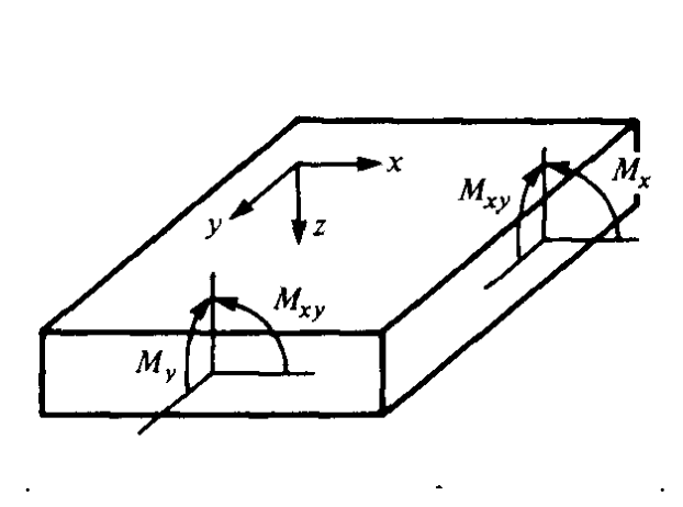
It will be convenient to normalize these tractions and moments by the width of the plate, so they have units of \(N/m\) and \(N-m/m\), or simply \(N\), respectively. Coordinates \(x\) and \(y\) are the directions in the plane of the plate, and \(z\) is customarily taken as positive downward. The deflection in the \(z\) direction is termed \(w\), also taken as positive downward.

Figure 5: Displacement of a point in a plate (from Powell, 1983).

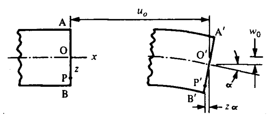
Analogously with the Euler assumption for beams, the Kirshchoff assumption for plate bending takes initially straight vertical lines to remain straight but rotate around the midplane (\(z = 0\)). As shown in Figure 5, the horizontal displacements \(u\) and \(v\) in the \(x\) and \(y\) directions due to rotation can be taken to a reasonable approximation from the rotation angle and distance from midplane, and this rotational displacement is added to the midplane displacement (\(u_0, v_0\)):

\[u = u_0 - z w_{0, x}\]

\[v = v_0 - z w_{0, y}\]

\[\epsilon = \left \{ \begin{array} {c} {\epsilon_x} \\ {\epsilon_y} \\ { \gamma_{xy}} \end{array} \right \} = \left \{ \begin{array} {c} {u_{,x}} \\ {v_{,y}} \\ {u_{,y} + v_{,x}} \end{array} \right \} = \left \{ \begin{array} {c} {u_{0,x} - zw_{0,xx}} \\ {v_{0,y} - zw_{0, yy}} \\ {(u_{0,y} + v_{0, x}) - 2z w_{0, xy}} \end{array} \right \} = \epsilon^0 + z\kappa\]

The strains are just the gradients of the displacements; using matrix notation these can be written where \(\epsilon^0\) is the midplane strain and \(\kappa\) is the vector of second derivatives of the displacement, called the curvature:

\(\kappa = \left \{ \begin{array} {c} {\kappa_x} \\ {\kappa_y} \\ { \kappa_{xy}} \end{array} \right \} = \left \{ \begin{array} {c} {-w_{0, xx}} \\ {-w_{0, yy}} \\ {-2w_{0, xy}} \end{array} \right \}\)

The component \(\kappa_{xy}\) is a twisting curvature, stating how the \(x\)-direction midplane slope changes with \(y\) (or equivalently how the \(y\)-direction slope changes with \(x\)).

The stresses relative to the \(x-y\) axes are now determined from the strains, and this must take consideration that each ply will in general have a different stiffness, depending on its own properties and also its orientation with respect to the \(x-y\) axes. This is accounted for by computing the transformed stiffness matrix \(\bar{D}\) as described in the previous section (Equation 4.4.11). Recall that the ply stiffnesses as given by Equation 4.4.4 are those along the fiber and transverse directions of that particular ply. The properties of each ply must be transformed to a common \(x-y\) axes, chosen arbitrarily for the entire laminate. The stresses at any vertical position are then:

\[\sigma = \bar{D} \epsilon = \bar{D} \epsilon^0 + z \bar{D} \kappa\]

where here \(\bar{D}\) is the transformed stiffness of the ply at the position at which the stresses are being computed.

Each of these ply stresses must add to balance the traction per unit width \(N\):

\[N = \int_{-h/2}^{+h/2} \sigma dz = \sum_{k = 1}^{N} \int_{z_k}^{z_{k + 1}} \sigma_k dz\]

where \(\sigma_k\) is the stress in the \(k\)th ply and \(z_k\) is the distance from the laminate midplane to the bottom of the \(k\)th ply. Using Equation 4.4.16 to write the stresses in terms of the mid-plane strains and curvatures:

\[N = \sum_{k = 1}^{N} (\int_{z_k}^{z_{k + 1}} \bar{D} \epsilon^0 dz + \int_{z_k}^{z_{k + 1}} \bar{D} \kappa z dz)\]

The curvature \(\kappa\) and midplane strain \(\epsilon^0\) are constant throughout \(z\), and the transformed stiffness \(\bar{D}\) does not change within a given ply. Removing these quantities from within the integrals:

\[N = \sum_{k = 1}^{N} (\bar{D} \epsilon^0 \int_{z_k}^{z_{k + 1}} dz + \bar{D} \kappa \int_{z_k}^{z_{k + 1}} z dz)\]

After evaluating the integrals, this expression can be written in the compact form:

\[N = \mathcal{A} \epsilon^0 + \mathcal{B} \kappa\]

where \(\mathcal{A}\) is an "extensional stiffness matrix" defined as:

\[\mathcal{A} = \sum_{k = 1}^{N} \bar{D} (z_{k + 1} - z_k)\]

and \(\mathcal{B}\) is a "coupling stiffness matrix" defined as:

\[\mathcal{B} = \dfrac{1}{2} \sum_{k = 1}^{N} \bar{D} (z_{k + 1}^2 - z_k^2)\]

The rationale for the names "extensional" and "coupling" is suggested by Equation 4.4.20. The \(\mathcal{A}\) matrix gives the inflfluence of an extensional mid-plane strain \(\epsilon^0\) on the inplane traction \(N\), and the \(\mathcal{B}\) matrix gives the contribution of a curvature \(\kappa\) to the traction. It may not be obvious why bending the plate will require an in-plane traction, or conversely why pulling the plate in its plane will cause it to bend. But visualize the plate containing plies all of the same stiffness, except for some very low-modulus plies somewhere above its midplane. When the plate is pulled, the more compliant plies above the midplane will tend to stretch more than the stiffer plies below the midplane. The top half of the laminate stretches more than the bottom half, so it takes on a concave-downward curvature.

Similarly, the moment resultants per unit width must be balanced by the moments contributed by the internal stresses:

\[M = \int_{-h/2}^{+h/2} \sigma z dz = \mathcal{B} \epsilon^0 + \mathcal{D} \kappa\]

where \(\mathcal{D}\) is a "bending stiffness matrix" defined as:

\[\mathcal{D} = \dfrac{1}{3} \sum_{k = 1}^{N} \bar{D} (z_{k + 1}^3 - z_k^3)\]

The complete set of relations between applied forces and moments, and the resulting midplane strains and curvatures, can be summarized as a single matrix equation:

\[\left \{ \begin{array} {c} {N} \\ {M} \end{array} \right \} = \begin{bmatrix} \mathcal{A} & \mathcal{B} \\ \mathcal{B} & \mathcal{D} \end{bmatrix} \left \{ \begin{array} {c} {\epsilon^0} \\ {\kappa} \end{array} \right \}\]

The \(\mathcal{A}/\mathcal{B}/\mathcal{B}/\mathcal{D}\) matrix in brackets is the laminate stiffness matrix, and its inverse will be the laminate compliance matrix.

The presence of nonzero elements in the coupling matrix \(\mathcal{B}\) indicates that the application of an in-plane traction will lead to a curvature or warping of the plate, or that an applied bending moment will also generate an extensional strain. These effects are usually undesirable. However, they can be avoided by making the laminate symmetric about the midplane, as examination of Equation 4.4.22 can reveal. (In some cases, this extension-curvature coupling can be used as an interesting design feature. For instance, it is possible to design a composite propeller blade whose angle of attack changes automatically with its rotational speed: increased speed increases the in-plane centripetal loading, which induces a twist into the blade.)

The above relations provide a straightforward (although tedious, unless a computer is used) means of determining stresses and displacements in laminated composites subjected to in-plane traction or bending loads:

1. For each material type in the stacking sequence, obtain by measurement or micromechanical estimation the four independent anisotropic parameters appearing in Equation 4.4.4: (\(E_1, E_2, \nu_{12}\), and \(G_{12}\)).

2. Using Equation 4.4.11, transform the compliance matrix for each ply from the ply's principal material directions to some convenient reference axes that will be used for the laminate as a whole.

3. Invert the transformed compliance matrix to obtain the transformed (relative to \(x-y\) axes) stiffness matrix. \(\bar{D}\).

4. Add each ply's contribution to the \(\mathcal{A}, \mathcal{B}\) and \(\mathcal{D}\) matrices as prescribed by Eqns. 4.4.21, 4.4.22 and 4.4.24.

5. Input the prescribed tractions \(N\) and bending moments \(M\), and form the system equations given by Equation 4.4.25.

6. Solve the resulting system for the unknown values of in-plane strain \(\epsilon^0\) and curvature \(\kappa\).

7. Use Equation 4.4.16 to determine the ply stresses for each ply in the laminate in terms of \(\epsilon^0, \kappa\) and \(z\). These will be the stresses relative to the \(x - y\) axes.

8. Use Equation 4.4.6 to transform the \(x - y\) stresses back to the principal material axes (parallel and transverse to the fibers).

9. If desired, the individual ply stresses can be used in a suitable failure criterion to assess the likelihood of that ply failing. The Tsai-Hill criterion is popularly used for this purpose:
   \[(\dfrac{\sigma_1}{\hat{\sigma}_1})^2 - \dfrac{\sigma_1 \sigma_2}{\hat{\sigma}_1^2} + (\dfrac{\sigma_2}{\hat{\sigma}_2})^2 + (\dfrac{\tau_{12}}{\hat{\tau}_{12}})^2 = 1\]
   Here \(\hat{\sigma}_1\) and \(\hat{\sigma}_2\) are the ply tensile strengths parallel to and onlong the fiber direction, and \(\hat{\tau}_{12}\) is the intralaminar ply strength. This criterion predicts failure whenever the left-hand-side of the above equation equals or exceeds unity.

Example \(\PageIndex{2}\)

The laminate analysis outlined above has been implemented in a code named plate, and this example demonstrates the use of this code in determining the stiffness of a two-ply 0/90 layup of graphite/epoxy composite. Here each of the two plies is given a thickness of 0.5, so the total laminate height will be unity. The laminate theory assumes a unit width, so the overall stiffness and compliance matrices will be based on a unit cross section.

> plate
assign properties for lamina type 1...

enter modulus in fiber direction... 
    (enter -1 to stop): 230e9
enter modulus in transverse direction: 6.6e9 
enter principal Poisson ratio: .25
enter shear modulus: 4.8e9
enter ply thickness: .5
assign properties for lamina type 2... 
enter modulus in fiber direction... 
    (enter -1 to stop): -1
define layup sequence, starting at bottom... 
    (use negative material set number to stop)
enter material set number for ply number 1: 1
enter ply angle: 0
enter material set number for ply number 2: 1
enter ply angle: 90
enter material set number for ply number 3: -1

laminate stiffness matrix:

    0.1185E+12  0.1653E+10  0.2942E+04   -0.2798D+11  0.0000D+00  0.7354D+03
    0.1653E+10  0.1185E+12  0.1389E+06    0.0000D+00  0.2798D+11  0.3473D+05
    0.2942E+04  0.1389E+06  0.4800E+10    0.7354D+03  0.3473D+05  0.0000D+00
    
   -0.2798E+11  0.0000E+00  0.7354E+03    0.9876D+10  0.1377D+09  0.2451D+03 
    0.0000E+00  0.2798E+11  0.3473E+05    0.1377D+09  0.9876D+10  0.1158D+05 
    0.7354E+03  0.3473E+05  0.0000E+00    0.2451D+03  0.1158D+05  0.4000D+09 

laminate compliance matrix: 
    
    0.2548E-10 -0.3554E-12 -0.1639E-16    0.7218D-10  0.7125D-19 -0.6022D-16 
   -0.3554E-12  0.2548E-10 -0.2150E-15    0.3253D-18 -0.7218D-10 -0.1228D-15 
   -0.1639E-16 -0.2150E-15  0.2083E-09   -0.6022D-16 -0.1228D-15  0.2228D-19 
   -0.6022E-16 -0.1228E-15  0.2228E-19   -0.1967D-15 -0.2580D-14  0.2500D-08 

Note that this unsymmetric laminate generates nonzero values in the coupling matrix \(\mathcal{B}\), as expected. The stiffness is equal in the \(x\) and \(y\) directions, as can be seen by examing the 1,1 and 2,2 elements of the laminate compliance matrix. The effective modulus is \(E_x = E_y = 1/0.2548 \times 10^{-10} = 39.2\) GPa. However, the laminate is not isotropic, as can be found by rerunning plate with the 0/90 layup oriented at a different angle from the \(x - y\) axes.

Temperature Effects

There are a number of improvements one might consider for the plate code described above: it could be extended to include interlaminar shear stresses between plies, it could incorporate a database of commercially available prepreg and core materials, or the user interface could be made \friendlier" and graphically-oriented. Many such features are available in commercial codes, or could be added by the user, and will not be discussed further here. However, thermal expansion effects are so important in application that a laminate code almost must have this feature to be usable, and the general approach will be outlined here.

In general, an increase in temperature \(\Delta T\) causes a thermal expansion given by the well-known relation \(\epsilon_T = \alpha \Delta T\), where \(\epsilon_T\) is the thermally-induced strain and \(\alpha\) is the coefficient of linear thermal expansion. This thermal strain is obtained without needing to apply stress, so that when Hooke's law is used to compute the stress from the strain the thermal component is subtracted first: \(\sigma = E(\epsilon - \alpha \Delta T)\). The thermal expansion causes normal strain only, so shearing components of strain are unaffected. Equation 4.4.3 can thus be extended as

where the thermal strain vector in the 1 - 2 coordinate frame is

\(\epsilon_T = \left \{ \begin{array} {c} {\alpha_1} \\ {\alpha_2} \\ {0} \end{array} \right \} \Delta T\)

Here \(\alpha_1\) and \(\alpha_2\) are the anisotropic thermal expansion coefficients in the fiber and transverse directions. Transforming to common \(x - y\) axes, this relation becomes:

\[\left \{ \begin{array} {c} {\sigma_x} \\ {\sigma_y} \\ {\tau_{xy}} \end{array} \right \} = \begin{bmatrix} \hat{D}_{11} & \hat{D}_{12} & \hat{D}_{13} \\ \hat{D}_{21} & \hat{D}_{22} & \hat{D}_{23} \\ \hat{D}_{31} & \hat{D}_{32} & \hat{D}_{33} \end{bmatrix} \left \{ \begin{bmatrix} {\epsilon_x} \\ {\epsilon_y} \\ {\epsilon_{xy}} \end{bmatrix} - \begin{bmatrix} {\alpha_x} \\ {\alpha_y} \\ {\alpha_{xy}} \end{bmatrix} \Delta T\right \}\]

The subscripts on the \(\bar{D}\) elements refer to row and column positions within the stiffness matrix rather than coordinate directions; the over-bar serves as a reminder that these elements refer to \(x - y\) axes. The thermal expansion vector on the right-hand side (\(\alpha = \alpha_x, \alpha_y, \alpha_{xy}\)) is essentially a strain vector, and so can be obtained from (\(\alpha_1, \alpha_2, 0\)) as in Equation 4.4.10:

\(\alpha = \left \{ \begin{array} {c} {\sigma_x} \\ {\sigma_y} \\ {\sigma_{xy}} \end{array} \right \} = RA^{-1} R^{-1} \left \{ \begin{array} {c} {\alpha_1} \\ {\alpha_2} \\ {0} \end{array} \right \}\)

Note that in the common \(x - y\) direction, thermal expansion induces both normal and shearing strains.

The previous temperature-independent development can now be repeated, modified only by carrying along the thermal expansion terms. As before, the strain vector for any position \(z\) from the midplane is given in terms of the midplane strain \(\epsilon^0\) and curvature \(\kappa\) by

\(\epsilon = \epsilon^0 + z\kappa\)

The corresponding stress is then

Balancing the stresses against the applied tractions and moments as before:

This result is identical to that of Equation 4.4.20 and Equation 4.4.23, other than the addition of the integrals representing the "thermal loads." This permits temperature-dependent problems to be handled by an "equivalent mechanical formulation;" the overall governing equations can be written as

\[\left \{ \begin{array} {c} \bar{N} & \bar{M} \end{array} \right \} = \begin{bmatrix} \mathcal{A} & \mathcal{B} \\ \mathcal{B} & \mathcal{D} \end{bmatrix} \left \{ \begin{array} {c} \epsilon^0 & \kappa \end{array} \right \}, \ \ \ or \ \ \ \left \{ \begin{array} {c} \epsilon^0 & \kappa \end{array} \right \} = \begin{bmatrix} \mathcal{A} & \mathcal{B} \\ \mathcal{B} & \mathcal{D} \end{bmatrix}^{-1} \left \{ \begin{array} {c} \bar{N} & \bar{M} \end{array} \right \}\]

where the \equivalent thermal loads" are given as

\(\bar{N} = N + \int \bar{D} \alpha \Delta T dz\)

\(\bar{M} = M + \int \bar{D} \alpha \Delta T z dz\)

The extension of the plate code to accommodate thermal effects thus consists of modifying the 6 \(\times\) 1 loading vector by adding the two 3 \(\times\) 1 vector integrals in the above expression.

Viscoelastic Effects

Since the matrix of many composite laminates is polymeric, the designer may need to consider the possibility of viscoelastic stress relaxation or creep during loading. Any such effect will probably not be large, since the fibers that bear most of the load are not usually viscoelastic. Further, the matrix material is usually used well below its glass transition temperature, and will act in a glassy elastic mode.

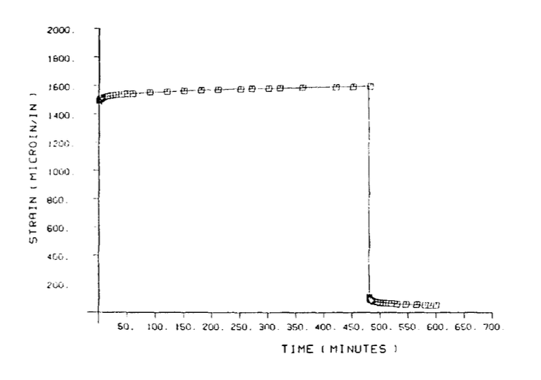
Some applications may not be so simple, however. If the laminate is used at elevated temperature, and if stresses act in directions not supported by the reinforcing fibers, relaxation effects may be observed. Figure 6 shows creep measured in a T300/5208 unidirectional graphite-epoxy laminate(M.E. Tuttle and H.F. Brinson, "Prediction of Long-Term Creep Compliance of General Composite Lami- nates," Experimental Mechanics, p. 89, March 1986.), loaded transversely to the fibers at 149\(^{\circ} C\). Even in this almost-worst case scenario, the creep strains are relatively small (less than 10% of the elastic strain), but Figure 6 does show that relaxation effects may be important in some situations.

Figure 6: Creep/creep-recovery response of graphite-epoxy laminate.

The Tuttle-Brinson paper cited above describes a time-stepping computational scheme that can be used to model these viscoelastic laminate effects, and a simplified form of their method will be outlined here. The viscoelastic creep strain occurring in a given ply during a time increment \(dt\) can be calculated from the stress in the ply at that time, assuming the ply to be free of adjoining plies; this gives an independent-ply creep strain. This strain will act to relax the ply stress.

Of course, the plies are not free to strain arbitrarily, and the proper strain compatibility can be reestablished by calculating the external loads that would produce elastic strains equal to the independent-ply creep strains. These loads are summed over all plies in the laminate to give an equivalent laminate creep load. This load is applied to the laminate to compute a set of compatible strains and curvatures, termed the equivalent-laminate creep strain. This strain is added to the initial elastic strain in computing the stress on a given ply, while the independent-ply creep strain is subtracted.

The following list develops these steps in more detail:

1. The elastic mid-plane strains and curvatures are solved for the specified bending moments and tractions, using the glassy moduli of the various plies. From Equation 4.4.25:

\(\left \{ \begin{array} {c} \epsilon^0 & \kappa \end{array} \right \} = \begin{bmatrix} \mathcal{A} & \mathcal{B} \\ \mathcal{B} & \mathcal{D} \end{bmatrix}^{-1} \left \{ \begin{array} {c} N & M \end{array} \right \}\)

2. The elastic strain in each ply is then obtained from Equation 4.4.15. For the \(k^{th}\) ply, with center at coordinate \(z\), this is:

\(\epsilon_{p\_e\_xy} = \epsilon^0 + z\kappa\)

where the \(p\_e\_xy\) subscript indicates ply, elastic, strain in the \(x-y\) direction. The elastic ply strains relative to the 1-2 (fiber-transverse) directions are given by the transformation of Equation 4.4.10:

\(\epsilon_{p\_e\_12} = RAR^{-1} \epsilon_{p\_e\_xy}\)

These first two steps are performed by the elastic plate code, and the adaptation to viscoelastic response consists of adding the following steps.

3. The current ply stress \(\sigma_{k\_12}\) in the 1-2 directions is:

The quantity \(\epsilon_{p\_lc\_12} - \epsilon_{p\_c\_12}\) is the difference between the equivalent laminate creep strain and the independent-ply creep strain. The quantities \(\epsilon_{p\_lc\_12}\) and \(\epsilon_{p\_c\_12}\) are set to zero initially, but are updated in steps 4 and 8 below to account for viscoelastic relaxation.

4. The current ply stress in then used in an appropriate viscoelastic model to compute the creep that would occur if the ply were free to strain independently of the adjoining plies; this is termed the independent ply creep strain. For a simple Voigt model, the current value of creep strain can be updated from its value in the previous time step as:

where the superscripts on strain indicate values at the current and previous time steps. Here \(C_v\) is the viscoelastic creep compliance and \(\tau\) is a relaxation time. A creep strain equal to \(C_v\) will develop in addition to the initial elastic strain in the laminate, and a fraction \(2/e\) of this creep strain will develop in a time \(\tau\). Different values of \(C_v\) will be used for the fiber, transverse, and shear strain components due to the anisotropy of the ply.

5. The stresses in the 1-2 and \(x-y) directions that would be needed to develop the independent- ply creep strains if the ply were elastic are

\(\sigma_{k\_12} = D\epsilon_{p\_c\_12}\)

\(\sigma_{k\_xy} = A^{-1} \sigma_{k\_12}\)

6. These equivalent elastic ply stresses are summed over all plies in the laminate to build up an equivalent laminate creep load. The contribution of the \(k^{th}\) ply is:

\(N_c = N_c + t_k \sigma_{k\_xy}\)

\(M_c = M_c + t_k z \sigma_{k\_xy}\)

where \(k^{th}\) is the thickness of the \(k^{th}\) ply and \(z\) is its centerline coordinate.

7. An equivalent laminate creep strain is then computed from the elastic compliance matrix and the equivalent laminate creep loads as

\(\left \{ \begin{array} {c} \epsilon_{lc}^0 & \kappa_{lc} \end{array} \right \} = \begin{bmatrix} \mathcal{A} & \mathcal{B} \\ \mathcal{B} & \mathcal{D} \end{bmatrix}^{-1} \left \{ \begin{array} {c} N_c & M_c \end{array} \right \}\)

8. The ply laminate creep strain in the \(x-y\) and 1-2 directions are

\(\epsilon_{p\_pc\_xy} = \epsilon_{lc}^0 + z \kappa_{lc}\)

\(\epsilon_{p\_lc\_12} = RAR^{-1} \epsilon_{p\_lc\_xy}\)

9. Finally, the time is incremented \((t \leftarrow t + dt)\) and another time cycle is computed starting at step 3.

Example \(\PageIndex{3}\)

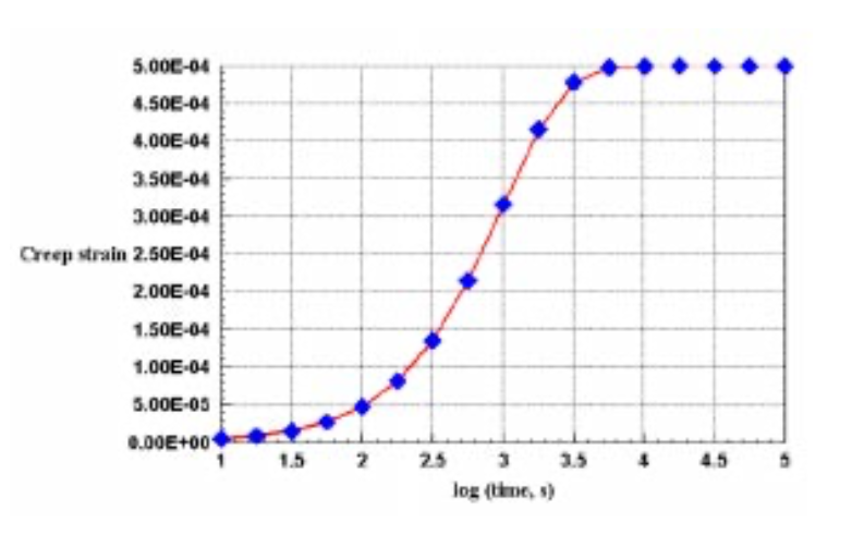
As an illustration of the above algorithm, consider a simple model laminate with one isotropic ply. The elastic constants are \(E = 100\) (arbitrary units) and \(\nu = 0.25\), and a unit stress is applied in the \(x\)-direction. The initial \(x\)-direction strain is therefore \(\epsilon_{x,0} = \sigma_x/E = 0.01\). In this isotropic test case, the code calculates the shear modulus as \(G = E/2(1 + \nu)\). The creep strain is governed by a parameter \(v_{frac}\), which sets the Voigt creep compliance \(G_v\) to \(v_{frac}/E_2\) in the transverse direction, \(v_{frac}/G_{12}\) for shear components, and zero in the fiber direction (assuming only elastic response along the fibers.)

Figure 7 shows the creep strain history of this laminate for a relaxation time of \(\tau = 1000\) s. The code steps linearly in log time, in this case with four time steps per decade. The creep strain is the strain over and beyond the initial elastic strain, which transitions from zero to \(C_v \epsilon_{x,0} = 5 \times 10^{-4}\) as time progresses through the relaxation time.

Figure 7: Creep strain history in model laminate.

References

1. Ashton, J.E., J.C. Halpin and P.H. Petit, Primer on Composite Materials: Analysis,Technomic Press, Westport, CT, 1969.

2. Jones, R.M., Mechanics of Composite Materials, McGraw-Hill, New York, 1975.

3. Powell, P.C, Engineering with Polymers, Chapman and Hall, London, 1983.

4. Roylance, D., Mechanics of Materials, Wiley & Sons, New York, 1996.

Exercise \(\PageIndex{1}\)

Write out the \(x-y\) two-dimensional compliance matrix \(\bar{S}\) and stiffness matrix \(\bar{D}\) (Equation 4.4.11) for a single ply of graphite/epoxy composite with its fibers aligned along the \(x-y\) axes.

Exercise \(\PageIndex{2}\)

Write out the \(x-y\) two-dimensional compliance matrix \(\bar{S}\) and stiffness matrix \(\bar{D}\) (Equation 4.4.11) for a single ply of graphite/epoxy composite with its fibers aligned 30\(^{\circ}\) from the \(x\) axis.

Exercise \(\PageIndex{3}\)

Plot the effective Young's modulus, measured along the \(x-\) axis, of a single unidirectional ply of graphite-epoxy composite as a function of the angle between the ply fiber direction and the \(x-\) axis.

Exercise \(\PageIndex{4}\)

Using a programming language of your choice, write a laminate code similar to the plate code mentioned in the text, and verify it by computing the laminate stiffness and compliance matrices given in Example \(\PageIndex{2}\).

Exercise \(\PageIndex{5}\)

A \((60^{\circ}/0^{\circ}/-60^{\circ})^S\) layup (the \(S\) superscript indicates the plies are repeated to give a symmetric laminate) is an example of what are called "quasi-isotropic" laminates, having equal stiffnesses in the \(x\) and \(y\) directions, regardless of the laminate orientation. Verify that this is so for two laminate orientations, one having the 0\(^{\circ}\) plies oriented along the \(x\) axis and the other with the 0\(^{\circ}\) plies oriented at 30\(^{\circ}\) from the \(x\) axis.

Mechanical Properties of Composite Materials

The following table lists physical and mechanical property values for representative ply and core materials widely used in fiber-reinforced composite laminates. Ply properties are taken from F.P.Gerstle, "Composites," Encyclopedia of Polymer Science and Engineering, Wiley, New York, 1991, which should be consulted for data from a wider range of materials. See also G. Lubin, Handbook of Composites, Van Nostrand, New York, 1982.

	S-glass/epoxy	Kevlar/epoxy	HM Graphite/epoxy	Pine	Rohacell 51 rigid foam
Elastic Properties: \(E_1\), GPa \(E_2\), GPa \(G_{12}\), GPa \(\nu_{12}\)	56 16 7.6 0.26	80 5.5 2.1 0.31	230 6.6 4.8 0.25	13.4 0.55 0.83 0.30	0.07 0.07 0.021
Tensile Strengths: \(\sigma_1\), MPa \(\sigma_2\), Mpa \(\sigma_{12}\), Mpa	1800 40 80	2000 20 40	1100 21 65	78 2.1 6.2	1.9 1.9 0.8
Compressive Strengths: \(\sigma_1\), MPa \(\sigma_2\), Mpa	690 140	280 140	620 170	33 3.0	0.9 0.9
Physical Properties: \(\alpha_1, 10^{-6}/^{\circ} C\) \(\alpha_2, 10^{-6}/^{\circ} C\) Volume fraction Thickness, \(mm\) Density, \(Mg/m^3\)	2.1 6.3 0.7 0.15 2.0	-4.0 60 0.54 0.13 1.38	-0.7 28 0.7 0.13 1.63	0.55	33 33 0.05