5.3: Finite Element Analysis

Introduction

Finite element analysis (FEA) has become commonplace in recent years, and is now the basis of a multibillion dollar per year industry. Numerical solutions to even very complicated stress problems can now be obtained routinely using FEA, and the method is so important that even introductory treatments of Mechanics of Materials – such as these modules – should outline its principal features.

In spite of the great power of FEA, the disadvantages of computer solutions must be kept in mind when using this and similar methods: they do not necessarily reveal how the stresses are influenced by important problem variables such as materials properties and geometrical features, and errors in input data can produce wildly incorrect results that may be overlooked by the analyst. Perhaps the most important function of theoretical modeling is that of sharpening the designer’s intuition; users of finite element codes should plan their strategy toward this end, supplementing the computer simulation with as much closed-form and experimental analysis as possible.

Finite element codes are less complicated than many of the word processing and spreadsheet packages found on modern microcomputers. Nevertheless, they are complex enough that most users do not find it effective to program their own code. A number of prewritten commercial codes are available, representing a broad price range and compatible with machines from microcomputers to supercomputers(C.A. Brebbia, ed., Finite Element Systems, A Handbook, Springer-Verlag, Berlin, 1982.). However, users with specialized needs should not necessarily shy away from code development, and may find the code sources available in such texts as that by Zienkiewicz(O.C. Zienkiewicz and R.L. Taylor, The Finite Element Method, McGraw-Hill Co., London, 1989.) to be a useful starting point. Most finite element software is written in Fortran, but some newer codes such as felt are in C or other more modern programming languages.

In practice, a finite element analysis usually consists of three principal steps:

1. Preprocessing: The user constructs a model of the part to be analyzed in which the geometry is divided into a number of discrete subregions, or "elements," connected at discrete points called "nodes." Certain of these nodes will have fixed displacements, and others will have prescribed loads. These models can be extremely time consuming to prepare, and commercial codes vie with one another to have the most user-friendly graphical "pre-processor" to assist in this rather tedious chore. Some of these preprocessors can overlay a mesh on a preexisting CAD file, so that finite element analysis can be done conveniently as part of the computerized drafting-and-design process.

2. Analysis: The dataset prepared by the preprocessor is used as input to the finite element code itself, which constructs and solves a system of linear or nonlinear algebraic equations

\(K_{ij} u_j = f_i\)

where \(u\) and \(f\) are the displacements and externally applied forces at the nodal points. The formation of the \(K\) matrix is dependent on the type of problem being attacked, and this module will outline the approach for truss and linear elastic stress analyses. Commercial codes may have very large element libraries, with elements appropriate to a wide range of problem types. One of FEA's principal advantages is that many problem types can be addressed with the same code, merely by specifying the appropriate element types from the library.

3. Postprocessing: In the earlier days of finite element analysis, the user would pore through reams of numbers generated by the code, listing displacements and stresses at discrete positions within the model. It is easy to miss important trends and hot spots this way, and modern codes use graphical displays to assist in visualizing the results. A typical postprocessor display overlays colored contours representing stress levels on the model, showing a full-field picture similar to that of photoelastic or moire experimental results

The operation of a specific code is usually detailed in the documentation accompanying the software, and vendors of the more expensive codes will often offer workshops or training sessions as well to help users learn the intricacies of code operation. One problem users may have even after this training is that the code tends to be a "black box" whose inner workings are not understood. In this module we will outline the principles underlying most current finite element stress analysis codes, limiting the discussion to linear elastic analysis for now. Understanding this theory helps dissipate the black-box syndrome, and also serves to summarize the analytical foundations of solid mechanics.

Matrix analysis of trusses

Pin-jointed trusses, discussed more fully in Module 5, provide a good way to introduce FEA concepts. The static analysis of trusses can be carried out exactly, and the equations of even complicated trusses can be assembled in a matrix form amenable to numerical solution. This approach, sometimes called “matrix analysis,” provided the foundation of early FEA development.

Matrix analysis of trusses operates by considering the stiffness of each truss element one at a time, and then using these stiffnesses to determine the forces that are set up in the truss elements by the displacements of the joints, usually called "nodes" in finite element analysis. Then noting that the sum of the forces contributed by each element to a node must equal the force that is externally applied to that node, we can assemble a sequence of linear algebraic equations in which the nodal displacements are the unknowns and the applied nodal forces are known quantities. These equations are conveniently written in matrix form, which gives the method its name:

\(\begin{bmatrix} K_{11} & K_{12} & \cdots & K_{1n} \\ K_{21} & K_{22} & \cdots & K_{2n} \\ \cdots & \cdots & \cdots & \cdots \\ K_{n1} & K_{n2} & \cdots & K_{nn} \end{bmatrix} \left \{ \begin{array} {c} u_1 \\ u_2 \\ \cdots \\ u_n \end{array} \right \} = \left \{ \begin{array} {c} f_1 \\ f_2 \\ \cdots \\ f_n \end{array} \right \}\)

Here \(u_i\) and \(f_j\) indicate the deflection at the ith node and the force at the \(j^{th}\) node (these would actually be vector quantities, with subcomponents along each coordinate axis). The \(K_{ij}\) coefficient array is called the global stiffness matrix, with the \(ij\) component being physically the influence of the \(j^{th}\) displacement on the \(i^{th}\) force. The matrix equations can be abbreviated as

\[K_{ij} u_j = f_i \text{ or } Ku = f\]

using either subscripts or boldface to indicate vector and matrix quantities.
Either the force externally applied or the displacement is known at the outset for each node, and it is impossible to specify simultaneously both an arbitrary displacement and a force on a given node. These prescribed nodal forces and displacements are the boundary conditions of the problem. It is the task of analysis to determine the forces that accompany the imposed displacements, and the displacements at the nodes where known external forces are applied.

Stiffness matrix for a single truss element

As a first step in developing a set of matrix equations that describe truss systems, we need a relationship between the forces and displacements at each end of a single truss element. Consider such an element in the \(x - y\) plane as shown in Figure 1, attached to nodes numbered \(i\) and \(j\) and inclined at an angle \(\theta\) from the horizontal.

Figure 1: Individual truss element.

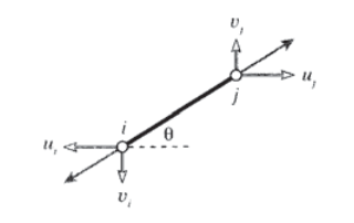
Considering the elongation vector \(\delta\) to be resolved in directions along and transverse to the element, the elongation in the truss element can be written in terms of the differences in the displacements of its end points:

where \(u\) and \(v\) are the horizontal and vertical components of the deflections, respectively. (The displacements at node \(i\) drawn in Figure 1 are negative.) This relation can be written in matrix form as:

\(\delta = \begin{bmatrix} -c & -s & c & s \end{bmatrix} \left \{ \begin{array} {c} u_i \\ v_i \\ u_j \\ v_j \end{array} \right \}\)

Here \(c = \cos \theta\) and \(s = \sin \theta\).

The axial force \(P\) that accompanies the elongation \(\delta\) is given by Hooke’s law for linear elastic bodies as \(P = (AE/L) \delta\). The horizontal and vertical nodal forces are shown in Figure 2; these can be written in terms of the total axial force as:

Figure 2: Components of nodal force.

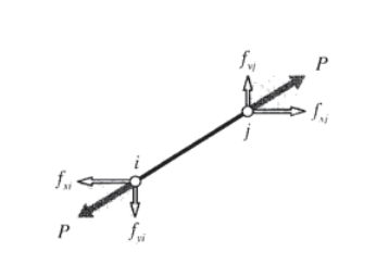
\(\left \{ \begin{array} {c} f_{xi} \\ f_{yi} \\ f_{xj} \\ f_{yj} \end{array} \right \} = \left \{ \begin{array} {c} -c \\ -s \\ c \\ s \end{array} \right \} P = \left \{ \begin{array} {c} -c \\ -s \\ c \\ s \end{array} \right \} \dfrac{AE}{L} \delta\)

\(= \left \{ \begin{array} {c} -c \\ -s \\ c \\ s \end{array} \right \} \dfrac{AE}{L} \begin{bmatrix} -c & -s & c & s \end{bmatrix} \left \{ \begin{array} {c} u_i \\ v_i \\ u_j \\ v_j \end{array} \right \}\)

Carrying out the matrix multiplication:

\[\left \{ \begin{array} {c} f_{xi} \\ f_{yi} \\ f_{xj} \\ f_{yj} \end{array} \right \} = \dfrac{AE}{L} \begin{bmatrix} c^2 & cs & -c^2 & -cs \\ cs & s^2 & -cs & -s^2 \\ -c^2 & -cs & c^2 & cs \\ -cs & -s^2 & cs & s^2 \end{bmatrix} \left \{ \begin{array} {c} u_i \\ v_i \\ u_j \\ v_j \end{array} \right \}\]

The quantity in brackets, multiplied by \(AE/L\), is known as the "element stiffness matrix" \(k_{ij}\). Each of its terms has a physical significance, representing the contribution of one of the displacements to one of the forces. The global system of equations is formed by combining the element stiffness matrices from each truss element in turn, so their computation is central to the method of matrix structural analysis. The principal difference between the matrix truss method and the general finite element method is in how the element stiffness matrices are formed; most of the other computer operations are the same.

Assembly of multiple element contributions

Figure 3: Element contributions to total nodal force.

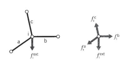
The next step is to consider an assemblage of many truss elements connected by pin joints. Each element meeting at a joint, or node, will contribute a force there as dictated by the displacements of both that element’s nodes (see Figure 3). To maintain static equilibrium, all element force contributions \(f_{i}^{elem}\) at a given node must sum to the force \(f_i^{ext}\) that is externally applied at that node:

\(f_i^{ext} = \sum_{elem} f_i^{elem} = (\sum_{elem} k_{ij}^{elem} u_j) = (\sum_{elem} k_{ij}^{elem}) u_j = K_{ij} u_j\)

Each element stiffness matrix \(k_{ij}^{elem}\) is added to the appropriate location of the overall, or "global" stiffness matrix \(K_{ij}\) that relates all of the truss displacements and forces. This process is called "assembly." The index numbers in the above relation must be the "global" numbers assigned to the truss structure as a whole. However, it is generally convenient to compute the individual element stiffness matrices using a local scheme, and then to have the computer convert to global numbers when assembling the individual matrices.

Example \(\PageIndex{1}\)

The assembly process is at the heart of the finite element method, and it is worthwhile to do a simple case by hand to see how it really works. Consider the two-element truss problem of Figure 4, with the nodes being assigned arbitrary "global" numbers from 1 to 3. Since each node can in general move in two directions, there are \(3 \times 2 = 6\) total degrees of freedom in the problem. The global stiffness matrix will then be a \(6 \times 6\) array relating the six displacements to the six externally applied forces. Only one of the displacements is unknown in this case, since all but the vertical displacement of node 2 (degree of freedom number 4) is constrained to be zero. Figure 4 shows a workable listing of the global numbers, and also "local" numbers for each individual element.

Figure 4: Global and local numbering for the two-element truss.

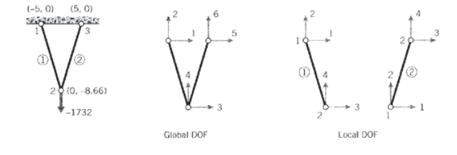
Using the local numbers, the \(4 \times 4\) element stiffness matrix of each of the two elements can be evaluated according to Equation 5.3.2. The inclination angle is calculated from the nodal coordinates as

The resulting matrix for element 1 is:

\(k^{(1)} = \begin{bmatrix} 25.00 & -43.30 & -25.00 & 43.30 \\ -43.30 & 75.00 & 43.30 & -75.00 \\ -25.00 & 43.30 & 25.00 & -43.30 \\ 43.30 & -75.00 & -43.30 & 75.00 \end{bmatrix} \times 10^3\)

and for element 2:

\(k^{(2)} = \begin{bmatrix} 25.00 & 43.30 & -25.00 & -43.30 \\ 43.30 & 75.00 & -43.30 & -75.00 \\ -25.00 & -43.30 & 25.00 & 43.30 \\ -43.30 & -75.00 & 43.30 & 75.00 \end{bmatrix} \times 10^3\)

(It is important the units be consistent; here lengths are in inches, forces in pounds, and moduli in psi. The modulus of both elements is \(E = 10\) Mpsi and both have area \(A = 0.1 in^2\).) These matrices have rows and columns numbered from 1 to 4, corresponding to the local degrees of freedom of the element.

However, each of the local degrees of freedom can be matched to one of the global degrees of the overall problem. By inspection of Figure 4, we can form the following table that maps local to global numbers:

local	global, element 1	global, element 2
1	1	3
2	2	4
3	3	5
4	4	6

Using this table, we see for instance that the second degree of freedom for element 2 is the fourth degree of freedom in the global numbering system, and the third local degree of freedom corresponds to the fifth global degree of freedom. Hence the value in the second row and third column of the element stiffness matrix of element 2, denoted \(k_{23}^{(2)}\), should be added into the position in the fourth row and fifth column of the \(6 \times 6\) global stiffness matrix. We write this as

\(k_{23}^{(2)} \to K_{4,5}\)

Each of the sixteen positions in the stiffness matrix of each of the two elements must be added into the global matrix according to the mapping given by the table. This gives the result

\(K = \begin{bmatrix} k_{11}^{(1)} & k_{12}^{(1)} & k_{13}^{(1)} & k_{14}^{(1)} & 0 & 0 \\ k_{21}^{(1)} & k_{22}^{(1)} & k_{23}^{(1)} & k_{24}^{(1)} & 0 & 0 \\ k_{31}^{(1)} & k_{32}^{(1)} & k_{33}^{(1)} + k_{11}^{(2)} & k_{34}^{(1)} + k_{12}^{(2)} & k_{13}^{(2)} & k_{14}^{(2)} \\ k_{41}^{(1)} & k_{42}^{(1)} & k_{43}^{(1)} + k_{21}^{(2)} & k_{44}^{(1)} + k_{22}^{(2)} & k_{23}^{(2)} & k_{24}^{(2)} \\ 0 & 0 & k_{31}^{(2)} & k_{32}^{(2)} & k_{33}^{(2)} & k_{34}^{(2)} \\ 0 & 0 & k_{41}^{(2)} & k_{42}^{(2)} & k_{43}^{(2)} & k_{44}^{(2)} \end{bmatrix}\)

This matrix premultiplies the vector of nodal displacements according to Equation 5.3.1 to yield the vector of externally applied nodal forces. The full system equations, taking into account the known forces and displacements, are then

Note that either the force or the displacement for each degree of freedom is known, with the accompanying displacement or force being unknown. Here only one of the displacements (\(u_4\)) is unknown, but in most problems the unknown displacements far outnumber the unknown forces. Note also that only those elements that are physically connected to a given node can contribute a force to that node. In most cases, this results in the global stiffness matrix containing many zeroes corresponding to nodal pairs that are not spanned by an element. Effective computer implementations will take advantage of the matrix sparseness to conserve memory and reduce execution time.

In larger problems the matrix equations are solved for the unknown displacements and forces by Gaussian reduction or other techniques. In this two-element problem, the solution for the single unknown displacement can be written down almost from inspection. Multiplying out the fourth row of the system, we have

\(0 + 0 + 0 + 150 \times 10^3 u_4 + 0 + 0 = -1732\)

\(u_4 = -1732/150 \times 10^3 = -0.01155 in\)

Now any of the unknown forces can be obtained directly. Multiplying out the first row for instance gives

\(0 + 0 + 0 + (43.4) (-0.0115) \times 10^3 + 0 + 0 = f_1\)

The negative sign here indicates the horizontal force on global node #1 is to the left, opposite the direction assumed in Figure 4.

The process of cycling through each element to form the element stiffness matrix, assembling the element matrix into the correct positions in the global matrix, solving the equations for displacements and then back-multiplying to compute the forces, and printing the results can be automated to make a very versatile computer code.

Larger-scale truss (and other) finite element analysis are best done with a dedicated computer code, and an excellent one for learning the method is available from the web at http://felt.sourceforge.net/. This code, named felt, was authored by Jason Gobat and Darren Atkinson for educational use, and incorporates a number of novel features to promote user-friendliness. Complete information describing this code, as well as the C-language source and a number of trial runs and auxiliary code modules is available via their web pages. If you have access to X-window workstations, a graphical shell named velvet is available as well.

Example \(\PageIndex{2}\)

Figure 5: The six-element truss, as developed in the velvet/felt FEA graphical interface.

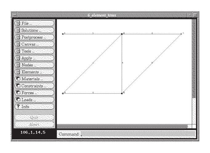
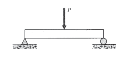
To illustrate how this code operates for a somewhat larger problem, consider the six-element truss of Figure 5, which was analyzed in Module 5 both by the joint-at-a-time free body analysis approach and by Castigliano’s method.

The input dataset, which can be written manually or developed graphically in velvet, employs parsing techniques to simplify what can be a very tedious and error-prone step in finite element analysis. The dataset for this 6-element truss is:

problem description
nodes=5 elements=6
nodes
1 x=0 y=100 z=0 constraint=pin
2 x=100 y=100 z=0 constraint=planar 3 x=200 y=100 z=0 force=P
4 x=0 y=0 z=0 constraint=pin
5 x=100 y=0 z=0 constraint=planar 
truss elements
1  nodes=[1,2]
2  nodes=[2,3]
3  nodes=[4,2]
4  nodes=[2,5]
5  nodes=[5,3]
6  nodes=[4,5]

material=steel
material properties steel E=3e+07 A=0.5

distributed loads

constraints
free Tx=u Ty=u Tz=u Rx=u Ry=u Rz=u 
pin Tx=c Ty=c Tz=c Rx=u Ry=u Rz=u 
planar Tx=u Ty=u Tz=c Rx=u Ry=u Rz=u

forces
P Fy=-1000

end 

The meaning of these lines should be fairly evident on inspection, although the felt documentation should be consulted for more detail. The output produced by felt for these data is:

** **

Nodal Displacements

Node #	DOF 1	DOF 2	DOF 3	DOF 4	DOF 5	DOF 6
1	0	0	0	0	0	0
2	0.013333	-0.03219	0	0	0	0
3	0.02	-0.084379	0	0	0	0
4	0	0	0	0	0	0
5	-0.0066667	-0.038856	0	0	0	0

Element Stresses

1:	4000
2:	2000
3:	-2828.4
4:	2000
5:	-2828.4
6:	-2000

Reaction Forces

Node #	DOF	Reaction Force
1	Tx	-2000
1	Ty	0
1	Tz	0
2	Tz	0
3	Tz	0
4	Tx	2000
4	Ty	1000
4	Tz	0
5	Tz	0

Material usage Summary

Material: steel
Number: 6
Length: 682.8427
Mass: 0.0000

Total mass: 0.0000

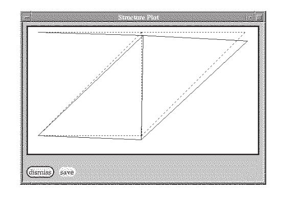
The vertical displacement of node 3 (the DOF 2 value) is -0.0844, the same value obtained by the closed-form methods of Module 5. Figure 6 shows the velvet graphical output for the truss deflections (greatly magnified).

Figure 6: The 6-element truss in its original and deformed shape.

General Stress Analysis

The element stiffness matrix could be formed exactly for truss elements, but this is not the case for general stress analysis situations. The relation between nodal forces and displacements are not known in advance for general two- or three-dimensional stress analysis problems, and an approximate relation must be used in order to write out an element stiffness matrix.

In the usual "displacement formulation" of the finite element method, the governing equations are combined so as to have only displacements appearing as unknowns; this can be done by using the Hookean constitutive equations to replace the stresses in the equilibrium equations by the strains, and then using the kinematic equations to replace the strains by the displacements. This gives

\[L^T \sigma = L^T D_{\epsilon} = L^T DLu = 0\]

Of course, it is often impossible to solve these equations in closed form for the irregular bound- ary conditions encountered in practical problems. However, the equations are amenable to discretization and solution by numerical techniques such as finite differences or finite elements.

Finite element methods are one of several approximate numerical techniques available for the solution of engineering boundary value problems. Problems in the mechanics of materials often lead to equations of this type, and finite element methods have a number of advantages in handling them. The method is particularly well suited to problems with irregular geometries and boundary conditions, and it can be implemented in general computer codes that can be used for many different problems.

To obtain a numerical solution for the stress analysis problem, let us postulate a function \(\tilde{u} (x, y)\) as an approximation to \(u\):

\[\tilde{u} (x, y) \approx u (x, y)\]

Many different forms might be adopted for the approximation \(\tilde{u}\). The finite element method discretizes the solution domain into an assemblage of subregions, or "elements," each of which has its own approximating functions. Specifically, the approximation for the displacement \(\tilde{u} (x, y)\) within an element is written as a combination of the (as yet unknown) displacements at the nodes belonging to that element:

\[\tilde{u} (x, y) = N_j (x, y) u_j\]

Here the index \(j\) ranges over the element’s nodes, \(u_j\) are the nodal displacements, and the \(N_j\) are “interpolation functions.” These interpolation functions are usually simple polynomials (generally linear, quadratic, or occasionally cubic polynomials) that are chosen to become unity at node \(j\) and zero at the other element nodes. The interpolation functions can be evaluated at any position within the element by means of standard subroutines, so the approximate displacement at any position within the element can be obtained in terms of the nodal displacements directly from Equation 5.3.5.

Figure 7: Interpolation in one dimension.

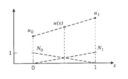
The interpolation concept can be illustrated by asking how we might guess the value of a function \(u(x)\) at an arbitrary point \(x\) located between two nodes at \(x = 0\) and \(x = 1\), assuming we know somehow the nodal values \(u(0)\) and u(1). We might assume that as a reasonable approximation \(u(x)\) simply varies linearly between these two values as shown in Figure 7, and write

Here the \(N_0\) and \(N_1\) are the linear interpolation functions for this one-dimensional approximation. Finite element codes have subroutines that extend this interpolation concept to two and three dimensions.

Approximations for the strain and stress follow directly from the displacements:

\[\tilde{\epsilon} L\tilde{u} = LN_ju_j \equiv B_j u_j\]

\[\tilde{\sigma} D \tilde{\epsilon} = DB_j u_j\]

where \(B_j(x, y) = LN_j (x, y)\) is an array of derivatives of the interpolation functions:

\[B_j = \begin{bmatrix} N_{j,x} & 0 \\ 0 & N_{j, y} \\ N_{j, y} & N_{j, x} \end{bmatrix}\]

A “virtual work” argument can now be invoked to relate the nodal displacement \(u_j\) appearing at node \(j\) to the forces applied externally at node \(i\): if a small, or "virtual," displacement \(\delta u_i\) is superimposed on node \(i\), the increase in strain energy \(\delta U\) within an element connected to that node is given by:

\[\delta U = \int_V \delta \epsilon^T \sigma dV\]

where \(V\) is the volume of the element. Using the approximate strain obtained from the interpolated displacements, \(\delta \tilde{\epsilon} = B_i \delta u_i\) is the approximate virtual increase in strain induced by the virtual nodal displacement. Using Equation 5.3.7 and the matrix identity \((AB)^T = B^T A^T\), we have:

\[\delta U = \delta u_i^T \int_V B_i^T DB_j dV u_j\]

(The nodal displacements \(\delta u_i^T\) and \(u_j\) are not functions of \(x\) and \(y\), and so can be brought from inside the integral.) The increase in strain energy \(\delta U\) must equal the work done by the nodal forces; this is:

\[\delta W = \delta u_i^T f_i\]

Equating Eqns. 5.3.10 and 5.3.11 and canceling the common factor \(\delta u_i^T\), we have

\[[\int_V B_i^T DB_j dV] u_j = f_i\]

This is of the disired form \(k_{ij} u_j = f_i\), where \(k_{ij} = \int_V B_i^T DB_j dV\) is the element stiffness.

Finally, the integral in Equation 12 must be replaced by a numerical equivalent acceptable to the computer. Gauss-Legendre numerical integration is commonly used in finite element codes for this purpose, since that technique provides a high ratio of accuracy to computing effort. Stated briefly, the integration consists of evaluating the integrand at optimally selected integration points within the element, and forming a weighted summation of the integrand values at these points. In the case of integration over two-dimensional element areas, this can be written:

\[\int_A f(x, y) dA \approx \sum_l f(x_l, y_l) w_l\]

The location of the sampling points \(x_l,y_l\) and the associated weights wl are provided by standard subroutines. In most modern codes, these routines map the element into a convenient shape, determine the integration points and weights in the transformed coordinate frame, and then map the results back to the original frame. The functions Nj used earlier for interpolation can be used for the mapping as well, achieving a significant economy in coding. This yields what are known as "numerically integrated isoparametric elements," and these are a mainstay of the finite element industry.

Equation 5.3.12, with the integral replaced by numerical integrations of the form in Equation 5.3.13, is the finite element counterpart of Equation 5.3.3, the differential governing equation. The computer will carry out the analysis by looping over each element, and within each element looping over the individual integration points. At each integration point the components of the element stiffness matrix \(k_{ij}\) are computed according to Equation 5.3.12, and added into the appropriate positions of the \(K_{ij}\) global stiffness matrix as was done in the assembly step of matrix truss method described in the previous section. It can be appreciated that a good deal of computation is involved just in forming the terms of the stiffness matrix, and that the finite element method could never have been developed without convenient and inexpensive access to a computer.

Stresses around a circular hole

We have considered the problem of a uniaxially loaded plate containing a circular hole in previous modules, including the theoretical Kirsch solution (Module 16) and experimental determinations using both photoelastic and moire methods (Module 17). This problem is of practical importance -- for instance, we have noted the dangerous stress concentration that appears near rivet holes -- and it is also quite demanding in both theoretical and numerical analyses. Since the stresses rise sharply near the hole, a finite element grid must be refined there in order to produce acceptable results.

Figure 8: Mesh for circular-hole problem.

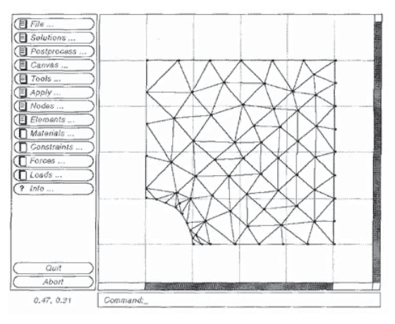
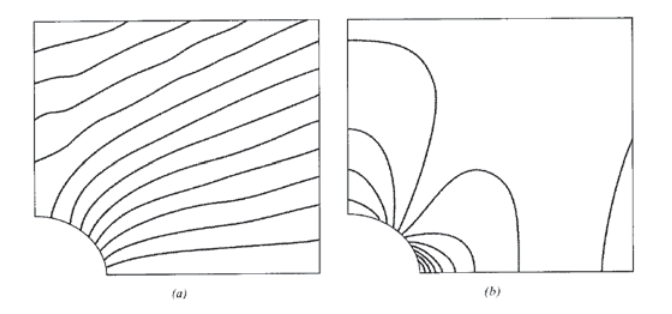
Figure 8 shows a mesh of three-noded triangular elements developed by the felt-velvet graphical FEA package that can be used to approximate the displacements and stresses around a uniaxially loaded plate containing a circular hole. Since both theoretical and experimental results for this stress field are available as mentioned above, the circular-hole problem is a good one for becoming familiar with code operation.

The user should take advantage of symmetry to reduce problem size whenever possible, and in this case only one quadrant of the problem need be meshed. The center of the hole is kept fixed, so the symmetry requires that nodes along the left edge be allowed to move vertically but not horizontally. Similarly, nodes along the lower edge are constrained vertically but left free to move horizontally. Loads are applied to the nodes along the upper edge, with each load being the resultant of the far-field stress acting along half of the element boundaries between the given node and its neighbors. (The far-field stress is taken as unity.) Portions of the felt input dataset for this problem are:

problem description
nodes=76 elements=116
nodes
1  x=1 y=-0 z=0 constraint=slide_x
2  x=1.19644 y=-0 z=0
3  x=0.984562 y=0.167939 z=0 constraint=free
4  x=0.940634 y=0.335841 z=0
5  x=1.07888 y=0.235833 z=0
.
.
.
72  x=3.99602 y=3.01892 z=0
73  x=3.99602 y=3.51942 z=0
74  x=3.33267 y=4 z=0
75  x=3.57706 y=3.65664 z=0
76 x=4 y=4 z=0
CSTPlaneStress elements
1  nodes=[13,12,23]
2  nodes=[67,58,55]
6  nodes=[50,41,40]
.
.
.
7  nodes=[68,67,69]
8  nodes=[68,58,67]
9  nodes=[57,58,68]
10 nodes=[57,51,58]
11  nodes=[52,51,57]
12  nodes=[37,39,52]
13 nodes=[39,51,52]
.
.
.
116 nodes=[2,3,1]

material properties
steel E=2.05e+11 nu=0.33 t=1

distributed loads
load_case_1 color=red direction=GlobalY values=(1,1) (3,1)
constraints
free Tx=u Ty=u Tz=u Rx=u Ry=u Rz=u
slide_x color=red Tx=u Ty=c Tz=c Rx=u Ry=u Rz=u 
slide_y color=red Tx=c Ty=u Tz=c Rx=u Ry=u Rz=u

end 

The \(y\)-displacements and vertical stresses σy are contoured in Figure 9(a) and (b) respectively; these should be compared with the photoelastic and moire analyses given in Module 17, Figs. 8 and 10(a). The stress at the integration point closest to the x-axis at the hole is computed to be \(\sigma_{y, \max} = 3.26\), 9% larger than the theoretical value of 3.00. In drawing the contours of Figure 9b, the postprocessor extrapolated the stresses to the nodes by fitting a least-squares plane through the stresses at all four integration points within the element. This produces an even higher value for the stress concentration factor, 3.593. The user must be aware that graphical postprocessors smooth results that are themselves only approximations, so numerical inaccuracy is a real possibility. Refining the mesh, especially near the region of highest stress gradient at the hole meridian, would reduce this error.

Figure 9: Vertical displacements (a) and stresses (b) as computed for the mesh of Figure 8.

Exercise \(\PageIndex{1}\)

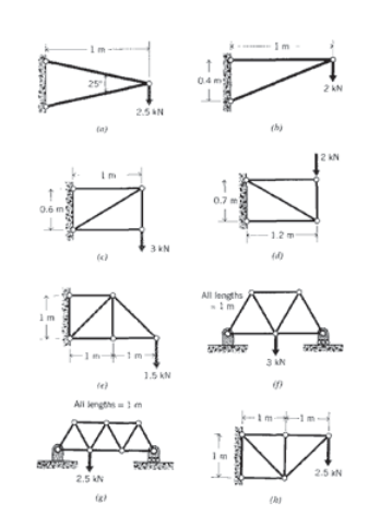
(a) – (h) Use FEA to determine the force in each element of the trusses drawn below.

Exercise \(\PageIndex{2}\)

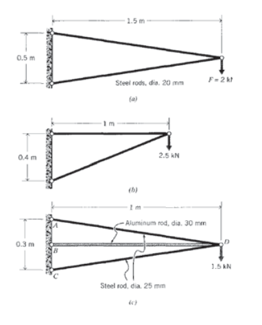
(a) – (c) Write out the global stiffness matrices for the trusses listed below, and solve for the unknown forces and displacements. For each element assume \(E = 30\) Mpsi and \(A = 0.1 in^2\).

Exercise \(\PageIndex{3}\)

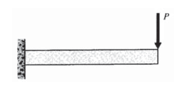
Obtain a plane-stress finite element solution for a cantilevered beam with a single load at the free end. Use arbitrarily chosen (but reasonable) dimensions and material properties. Plot the stresses \(\sigma_x\) and \(\tau_{xy}\) as functions of \(y\) at an arbitrary station along the span; also plot the stresses given by the elementary theory of beam bending (c.f. Module 13) and assess the magnitude of the numerical error.

Exercise \(\PageIndex{4}\)

Repeat the previous problem, but with a symmetrically-loaded beam in three-point bending.

Exercise \(\PageIndex{5}\)

Use axisymmetric elements to obtain a finite element solution for the radial stress in a thick-walled pressure vessel (using arbitrary geometry and material parameters). Compare the results with the theoretical solution (c.f. Prob. 2 in Module 16).