6.1: Constitutive and Governing Relations

Surface waves in water are a superb example of a stationary and ergodic random process. The model of waves as a nearly linear superposition of harmonic components, at random phase, is confirmed by measurements at sea, as well as by the linear theory of waves, the subject of this section. We will skip some elements of fluid mechanics where appropriate, and move quickly to the cases of two-dimensional, inviscid and irrotational flow. These are the major assumptions that enable the linear wave model.

First, we know that near the sea surface, water can be considered as incompressible, and that the density \(\rho\) is nearly uniform. In this case, a simple form of conservation of mass will hold:

\[ \dfrac{\partial u}{\partial x} + \dfrac{\partial v}{\partial y} + \dfrac{\partial w}{\partial z} = 0; \]

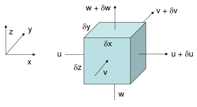
where the Cartesian space is \([x, \, y, \, z]\), with respective particle velocity vectors \([u, \, v, \, w]\). In words, the above equation says that net flow into a differential volume has to equal net flow out of it. Considering a box of dimensions \( [\delta x, \, \delta y, \, \delta z] \), we see that any \(\delta u\) across the \(x\)-dimension has to be accounted for by \(\delta v\) and \(\delta w\):

\[ \delta u\, \delta y\, \delta z + \delta v\, \delta z\, \delta z + \delta w\, \delta x\, \delta y = 0. \]

Figure \(\PageIndex{1}\): illustrates the relationship between the 3-dimensional Cartesian coordinate system and its associated unit vectors.

Next, we invoke Newton’s law, in the three directions:

\begin{align} \rho \left[ \dfrac{\partial u}{\partial t} + u \dfrac{\partial u}{\partial x} + v \dfrac{\partial u}{\partial y} + w \dfrac{\partial u}{\partial z} \right] \, &= \, -\dfrac{\partial p}{\partial x} + \mu \left[ \dfrac{\partial^2 u}{\partial x^2} + \dfrac{\partial^2 u}{\partial y^2} + \dfrac{\partial^2 u}{\partial z^2} \right]; \\[4pt] \rho \left[ \dfrac{\partial v}{\partial t} + v \dfrac{\partial v}{\partial x} + w \dfrac{\partial v}{\partial y} + u \dfrac{\partial v}{\partial z} \right] \, &= \, -\dfrac{\partial p}{\partial y} + \mu \left[ \dfrac{\partial^2 v}{\partial x^2} + \dfrac{\partial^2 v}{\partial y^2} + \dfrac{\partial^2 v}{\partial z^2} \right]; \\[4pt] \rho \left[ \dfrac{\partial w}{\partial t} + w \dfrac{\partial w}{\partial x} + u \dfrac{\partial w}{\partial y} + v \dfrac{\partial w}{\partial z} \right] \, &= \, -\dfrac{\partial p}{\partial z} + \mu \left[ \dfrac{\partial^2 x}{\partial x^2} + \dfrac{\partial^2 w}{\partial y^2} \dfrac{\partial^2 w}{\partial z^2} \right] - \rho g. \end{align}

Here the left-hand side of each equation is the acceleration of the fluid particle, as it moves through the differential volume. The terms such as \(u \frac{\partial u}{\partial x}\) capture the fact that the force balance is for a moving particle; the chain rule expansion goes like this in the \(x\)-direction:

\[ \dfrac{du}{dt} = \dfrac{\partial u}{\partial t} + \dfrac{\partial u}{\partial x} \dfrac{\partial x}{\partial t} + \dfrac{\partial u}{\partial y} \dfrac{\partial y}{\partial t} + \dfrac{\partial u}{\partial z} \dfrac{\partial z}{\partial t}, \]

where \(u = \partial x / \partial t\) and so on.

On the right side of the three force balance equations above, the differential pressure clearly acts to slow the particle (hence the negative sign), and viscous friction is applied through absolute viscosity \(\mu\). The third equation also has a term for gravity, leading in the case of zero velocities to the familiar relation \(p(z) = - \rho g z\), where \(z\) is taken positive upward from the mean free surface.