
7.4: Linear Programming
- Page ID
- 47261

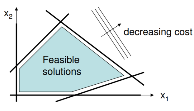
We now consider the case that the cost is a linear function of \(n\) parameters. There is clearly no solution unless the parameter space is constrained, and indeed the solution is guaranteed to be on the boundary. The situation is well illustrated in two dimensions \((n = 2)\), an example of which is shown below. Here, five linear inequality boundaries are shown; no \(x\) are allowed outside of the feasible region. In the general case, both equality and inequality constraints may be present.
.png?revision=1)
The nature of the problem - all linear, and comprising inequality and possibly equality constraints - admits special and powerful algorithms that are effective even in very high dimensions, e.g., in the thousands. In lower dimensions, we can appeal to intuition gained from the figure to construct a simpler method for small systems, say up to ten unknowns.
Foremost, it is clear from the figure that the solution has to lie on one of the boundaries. The solution in fact lies at a vertex of \(n\) hypersurfaces of dimension \(n-1\). Such a hypersurface is a line in two-dimensional space, a plane in three-space, and so on. We will say that a line in three-space is an intersection of two planes, and hence is equivalent to two hypersurfaces of dimension two. It can be verified that a hypersurface of dimension \(n-1\) is defined with one equation.
If there are no equality constraints, then these \(n\) hypersurfaces forming the solution vertex are a subset of the \(I\) inequality constraints. We will generally have \(I>n\). If there are also \(E<n\) equality constraints, then the solution lies at the intersection of these \(E\) equality hypersurfaces and \(n-E\) other hypersurfaces taken from the \(I\) inequality constraints. Of course, if \(E=n\), then we have only a linear system to solve. Thus we have a combinatorics problem; consider the case of inequalities only, and then the mixed case.
- \(I\) inequalities, no equalities. \(n\) of the inequalities will define the solution vertex. The number of combinations of \(n\) constraint equations among \(I\) choices is \(I!/(I −n)!n!\). Algorithm: For each combination (indexed \(k\), say) in turn, solve the linear system of equations to find a solution \(x_k\). Check that the solution does not violate any of the other \(I-n\) inequality constraints. Of all the solutions that are feasible (that is, they do not violate any constraints), pick the best one - it is optimal.
- \(I\) inequalities, \(E\) equalities. The solution involves all the equalities, and \(n-E\) inequality constraints. The number of combinations of \(n-E\) constraint equations among \(I\) choices is \(I! / (I-n+E)! (n-E)!\). Algorithm: For each combination (indexed with \(k\)) in turn, solve the linear set of equations, to give a candidate solution \(x_k\). Check that the solution does not violate any of the remaining \(I-n+E\) inequality constraints. Of all the feasible solutions, pick the best one - it is optimal.
The above rough recipe assumes that none of the hypersurfaces are parallel; parallel constraints will not intersect and no solution exists to the linear set of equations. Luckily such cases can be detected easily (e.g., by checking for singularity of the matrix), and classified as infeasible. In the above figure, \(I = 5\) and \(n = 2\). Hence there are \(5!/(5-2)!2! = 10\) combinations to try: AB, AC, AD, AE, BC, BD, BE, CD, CE, DE. Only five are evident, because some of the intersections are outside of the area indicated (Can you find them all?).
The linear programming approach is extremely valuable in many areas of policy and finance, where costs scale linearly with quantity, and inequalities are commonplace. There are also a great many engineering applications, because of the prevalence of linear analysis.