7.5: Integer Linear Programming

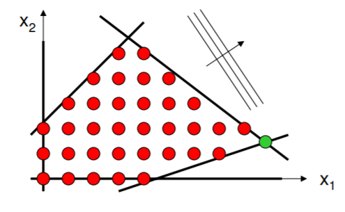
Sometimes the constraint and cost functions are continuous, but only integer solutions are allowed. Such is the case in commodities markets, where it is expected that one will deal in tons of butter, whole automobiles, and so on. The image below shows integer solutions within a feasible domain defined by continuous function inequalities. Note that the requirement of an integer solution makes it far less obvious how to select the optimum point; it is no longer a vertex.

Figure 7.3.1, where only integer values that fall within the bounded region are allowed solutions. The solution identified in last section, marked in green, is not an integer and thus no longer an acceptable solution.

The branch-and-bound method comes to the rescue. In words, what we will do is successively solve continuous linear programming problems, but while imposing new inequality constraints that force the elements into taking integer values.

The method uses two major concepts. The first has to do with bounds and is quite intuitive. Suppose that in a solution domain \(X_1\), the cost has a known upper bound \(\bar{f}_1\), and that in a different domain \(X_2\), the cost has a known lower bound \(\underline{f}_1\). Suppose further that \(\bar{f}_1 < \underline{f}_2\). If it is desired to minimize the function, then such a comparison clearly suggests we need spend no more time working in \(X_2\). The second concept is that of a branching tree, and an example is the best way to proceed here. We try to maximize\(^1\)

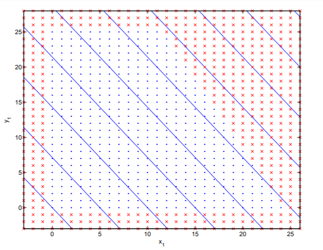
\begin{align*} J \, &= \, 1000 x_1 + 700 x_2, \textrm{ subject to} \\[4pt] 100 x_1 + 50 x_2 \, &\leq \, 2425 \textrm { and} \\[4pt] x_2 \, &\leq \, 25.5. \\[4pt] &\ \quad \textrm{with both \(x_1, \, x_2\) positive integers} \end{align*}

Figure \(\PageIndex{2}\): the range of possible integer values for solutions to this problem, with allowed values indicated by blue dots.

Hence we have four inequality constraints; the problem is not dissimilar to what is shown in the above figure. First, we solve the continuous linear programming problem, finding

\[ A: \, J = 29350 \, : \, x_1 = 11.5, \, x_2 = 25.5 \nonumber \] Clearly, because neither of the solution elements is an integer, this solution is not valid. But it does give us a starting point in branch and bound: Branch this solution into two, where we consider the integers \(x_2\) closest to \(25.5\):

\begin{align*} B: \, J(x_2 \leq 25) \, &= \, 29250 \, : \, x_1 = 11.75, \, x_2 = 25 \textrm{ and} \\[4pt] C: \, J(x_2 \geq 26) \, &= \, X, \end{align*}

where the \(X\) indicates we have violated one of our original constraints. So there is nothing more to consider along the lines of \(C\). But we pursue \(B\) because it still has non-integer solutions, branching \(x_1\) into

\begin{align*} D: \, J(x_1 \leq 11, \, x_2 \leq 25) \, &= \, 28500 \, : \, x_1 = 11, x_2 = 25 \textrm{ and} \\[4pt] E: \, J(x_1 \geq 11, \, x_2 \leq 25) \, &= \, 29150 \, : \, x_1 = 12, x_2 = 24.5. \end{align*}

\(D\) does not need to be pursued any further, since it is has integer solutions; we store \(D\) as a possible optimum. Expanding \(E\) in \(x_2\), we get

\begin{align*} F: \, J(x_1 \geq 12, \, x_2 \leq 24) \, &= \, 29050 \, : \, x_1 = 12.25, \, x_2 = 24, \textrm { and} \\[4pt] G: \, J(x_1 \geq 12, \, x_2 \leq 25) \, &= \, X. \end{align*}

\(G\) is infeasible because it violates one of our original inequality constraints, so this branch dies. \(F\) has non-integer solutions so we branch in \(x_1\):

\begin{align*} H: \, J(x_1 \leq 12, \, x_2 \leq 24) \, &= \, 28800 \, : \, x_1 = 12, \, x_2 = 24 \textrm { and} \\[4pt] I: \, J(x_1 \geq 13, \, x_2 \leq 24) \, &= \, 28750 \, : \, x_1 = 13, \, x_2 = 22.5. \end{align*}

Now \(I\) is a non-integer solution, but even so it is not as good as \(H\), which does have an integer solution, so there is nothing more to pursue from \(I\). \(H\) is better than \(D\), the other available integer solution - so it is the optimal.

Figure \(\PageIndex{3}\): visual representation of the reasoning behind the branch-and-bound method. Values that fall outside the allowed bounds are abandoned and marked in red; viable branch points are in white; solutions that satisfy all the conditions are marked in pale orange for later comparison, with blue marking the optimal among these possible solutions.

There exist many commercial programs for branch-and-bound solutions of integer linear programming problems. We implicitly used the upper-vs.-lower bound concept in terminating at \(I\): if a non-integer solution is dominated by any integer solution, no branches from it can do better either.

---

\(^{\PageIndex{1}}\): This problem is from G. Sierksma, Linear and integer programming, Marcel Dekker, New York, 1996.