Chapter 8: Polymers and Soft Matter

8.1 Soft Matter

I have recorded a series of videos to supplement this text which can be found in the playlist below:

https://www.youtube.com/playlist?lis...4HrNeEDCchR8V1

Soft materials is a class of materials that includes polymers, colloids, liquid crystals, nanoparticles, and hybrid organic-inorganic materials systems. We are primarily going to focus on polymers but the governing physics and foundation that we will develop will apply more broadly to soft materials and be particularly relevant to biological systems as well as most biological systems are composed primarily of soft materials.

The key to the interesting properties of soft matter is that most intermolecular interactions in soft matter systems have energies (enthalpies) on the scale of approximately 1 kT. By comparison, most hard materials such as metals or ceramics are held together by much stronger covalent bonds, which have energetic interactions on the order of 10-100 kT. In other words, soft matter is held together by very weak intermolecular interactions, which leads to large fluctuations in thermodynamic quantities that determine the interesting physical behavior of polymer systems. In particular, this means that intermolecular bonds can be easily broken by applied stimuli, such as a pulling force. One consequence of the prevalence of weak intermolecular bonds is that soft matter is highly adaptive, meaning that systems can undergo significant changes in response to stimuli. Adaptive behavior is particularly prominent in biological systems. For example, many proteins, such as transporters or receptors, rely on large conformational changes that are only possible in soft matter systems because bonding interactions are relatively weak. That said, soft matter systems can still be strong and robust with respect to physical stimuli, since very strong properties can be built up from a very large number of weak interactions. For example, Kevlar, a prominent synthetic polymer, is used in bulletproof vests due to its ability to withstand impact, a property derived from a large number of weak interactions that are enhanced by the structure of the Kevlar backbone. The physical consequences of these weak enthalpic interactions will become more apparent when we start discussing the thermodynamics of polymeric systems in future lectures. As we continue in the class we will also clarify the origin of different types of bonds, the impact of molecular geometry and structure, the role of fluctuations in position and conformation, and the interplay of enthalpy and entropy over several important length scales.

Throughout the study of soft matter, we will be interested in understanding polymeric behavior on different length scales, or equivalently, we will be interested in hierarchical behavior. This is due to the multitude to length scales associated with soft matter systems. Typically, we can think of bonding behavior as relevant on the Angstrom or nanometer length scale, while selfassembled biological structures such as DNA, viruses, and cellular components have properties associated with the 10s to 100s of nanometers, or even up to the micrometer length scale.

What we will find, though, is that the properties of soft matter relies on the bridging of length scales - polymers that have widths on the order of nanometers, but lengths of up to meters. It is a challenge to study systems across these length scales, and is unusual in the study of hard materials!

8.2 Polymer Chain Conformations:

We now know how to create polymers and we have discussed some of the unique characteristics of polymer chains (inter vs intramolecular bonding). We also have seen some of the different polymer architectures that we will encounter but we haven’t really talked much about polymer conformations. I make a distinction here between architecture and conformation. Polymer architecture has a connotation referring to the the structure of the polymer whereas a polymer chain conformation has a connotation which refers to the instantaneous state of the polymer especially when subjected to an external stimuli.

In our discussion of polymer chain conformations we will start simple and build up from a simple homopolymer with a very high molecular weight. So this polymer architecture is simply linear, flexible, chain or if you like macroscopic analogies spaghetti. And the flexibility of the chain will be governed by the intramolecular bonding of the repeat unit, as well as other factors which we will get into in depth when we discuss the glass transition temperature. One of the key ways that we can characterize a polymer chain conformation, just like we did with molar mass in the previous lecture, is by describing the effective size of a single polymer chain in solution. Now you might reasonably think that the size of a linear polymer chain is simply the length of the monomer or repeat unit multiplied by the number of repeat units. However, this is not the case as we are interested in the effective size of the polymer which is the space occupied by the polymer. We will see in this lecture that depending on the temperature, solvent, and local environment even this simple polymer chain can adopted a highly coiled collapsed structure, an highly elongated structure, or even in the most extreme circumstances a fully elongated structure. We also know from our supplemental thermodynamics notes that polymers can adopt a large number of possible conformation, microstates. The conformation and thus the effective size of the polymer can change rapidly. This means that we will also have to develop a metric to measure the size of the polymer which is probabilistic in nature.

You can see this in the embedded video in the PowerPoint slides.

We will describe in detail several different models which will describe the effective size of polymers with increasing complexity

• Ideal/Freely Jointed Chain Model

• Mathematician’s Ideal Chain

• Chemist’s Chain in Solution and Melt Model

• Physicist’s Ideal Chain

We will examine the differences in each model and how the scaling changes depending on some of the factors mentioned above.

8.2.1 Characterizing Polymer Size: Mean-Squared-Displacement

We have just mentioned that describing the effective size of the polymer can be tricky and it is not just a matter of adding up the monomer lengths. This problem becomes even more complex when we are dealing with polymers with a more complex architecture, i.e. branched, dendrimer, star polymers, syndiotactic, etc. How do we characterize the size of a polymer then? Well the tool that we will use is the root mean squared end to end distance (RMSD) which is shown below

\begin{equation}
\langle r^{2} \rangle ^{\frac{1}{2}}
\end{equation}

where r is the vectorial position of the polymer at one end and the other end in 3D, seen in the image below

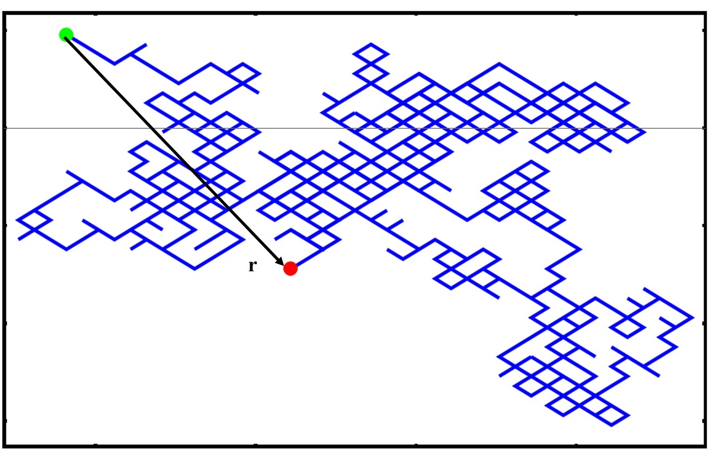
We take the square because this will give us a quantity in units of length. Note as well that the ⟨⟩ indicates an average quantity as we will typically average over many microstates and conformations. You can also see that by squaring the r we will never have negative values. Now there are many ways of calculating a mean square displacement. One method is simply averaging the end-to-end displacement values of a single polymer chain as it moves and fluctuates over time or you can average one snapshot of identical polymer chains which are all under the same external stimuli/experimental conditions.

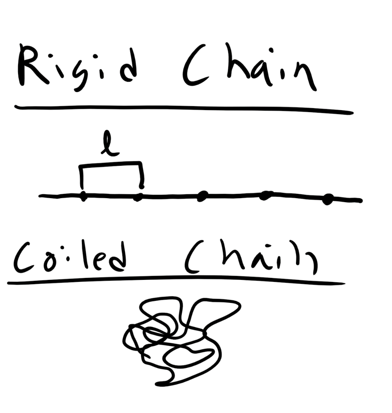
To get started let’s do a quick couple of extreme example of a linear rigid rod like polymer architecture that is stretched to the fully extended position. This polymer has a monomer length of l and the number of monomers is as always n. What is the MSD end-to-end distance?

Well let’s start with the r vector?

It is nl ! So

\begin{equation}
\langle r^2 \rangle ^{\frac{1}{2}} = nl = L
\end{equation}

where L is the contour length of the polymer, the fully extended distance.

8.2.2 Ideal/Freely Jointed Chain (FJC)/Gaussian Model

Now the above example is an very extreme situation, although an important one to consider. However, polymers are not typically fully extended and this is an energetically unfavorable microstate. To describe a more typical polymer conformation let’s start with a simpler model. Let’s consider an ideal polymer chain where we assume that there are no intramolecular steric interactions along the polymer chain. This means that the polymer can intersect itself along the backbone without any penalty. This is the Ideal/FJC/Gaussian Chain Model.

So again here we have a polymer chain with a monomer length, l, and a number of monomers, n. We also assume that in addition to the ability of chain to cross over itself the monomers can rotate in any dimension with respect to one another. We are essentially ignoring the constraints that double or triple carbon bonds can place on polymer rotation, steric or repulsive interactions, or intermolecular interactions. So with all of these assumptions we can describe the polymer as essentially performing a random walk through space in time. Or alternatively we can construct a polymer chain by placing each monomer in a position in space using a stochastic or random algorithm (Monte Carlo). In this random walk the step size would be fixed at l from the previous step/monomer and would continue until reaching n random steps. Thus the position of monomer i and i+1 are completely uncorrelated.

8.2.3 Mathematician’s Ideal Chain Derivation for Ideal Chain/FJC Model

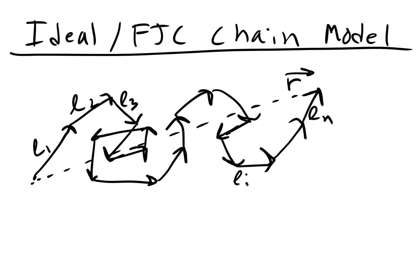
We can derive the MSD of of the FJC Chain model without using a probabilistic perspective as well and this might be a little more intuitive for some people, at least it was for me. Again remember that in the random walk or ideal model we ignore bonding and it is really unphysical in most cases. The end-to-end distance of the Ideal Chain/FJC model can be derived using a different mathematical formalism, sometimes referred to as the Mathematician’s Ideal Chain. We again assume n monomers with a fixed monomer length l and which is represented as a vector in 3D space \(\vec{l_i}\)where this vector refers to monomer i.

So the end to end distance vector is

\begin{equation}
\vec{r} = \vec{l_1} + \vec{l_2} + ... +\vec{l_n} = \sum_{i=1}^{n} \vec{l_{i}}
\end{equation}

On average what will be the value of \(\langle \vec{r} \rangle\)? Remember that for the ideal polymer chain each step positive or negative is equally likely, these steps are uncorrelated. So on average the value of \(\langle \vec{r} \rangle\) = 0.

The better question is what will be \(\langle \vec{r}^2 \rangle\) and we can write this as the dot product

\begin{equation}
\langle \vec{r}_{i} \cdot \vec{r}_{j} \rangle = \bigg \langle \sum_{i=1}^{n} \vec{l}_{i} \cdot \sum_{j=1}^{n} \vec{l}_{j} \bigg \rangle
\end{equation}

where i and j refer to monomer i and monomer j. Remember that the dot product is

\begin{equation}
\vec{l}_{i} \cdot \vec{l}_{j} = |l_{i}||l_{j}| \cos \theta_{ij}
\end{equation}

We can show the MSD in matrix notation as well

\[
\langle\vec{r}_i \cdot \vec{r}_j \rangle =
\left [ {\begin{array}{ccccc}
\vec{l_1}\cdot\vec{l_1} & \vec{l_1}\cdot\vec{l_2} & \vec{l_1}\cdot\vec{l_3} & \ldots & \vec{l_1}\cdot\vec{l_n} \\
\vec{l_2}\cdot\vec{l_1} & \vec{l_2}\cdot\vec{l_2} & \ldots \\
\vdots & & & \ddots \\ \\
\vec{l_n}\cdot\vec{l_1} & \ldots & & & \vec{l_n}\cdot\vec{l_n} \\
\end{array} } \right ]
\]

Now let’s think about the value of the dot product on the diagonal component. The magnitude will simply be \(l^2\) for every component but now we need to think about the cosθ between the two vectors. Well for the diagonal component they will always be pointing in the same direction so the angle will be 0^o and then cos0^o = 1.

Now for the off diagonal components. Let’s keep it simple and think about the 1D scenario. Well there the value of cosθ = 1 or = −1. But remember we are concerned about the averages so since both positive and negative steps are equally probable (Markov/Monte Carlo) or uncorrelated so on average the value of cosθ = 0.

So the matrix reduces to

\[
\langle\vec{r}_i \cdot \vec{r}_j \rangle =
\left[ {\begin{array}{ccccc}
l^2 & 0 & 0 & \ldots & 0 \\
0 &l^2 & \ldots \\
\vdots & & & \ddots \\ \\
0 & \ldots & & & l^2 \\
\end{array} } \right]
\]

The sum of this matrix becomes

\begin{equation}
\langle r^2 \rangle = nl^2
\end{equation}

just as we obtained previously with our other probabilistic method!

8.3 The Chemist’s Polymer Chain Model

So far we have neglected a lot of detail in describing polymer chains that make the previous models a bit unphysical. We have neglected taking into account restrictions in bond angles to to steric hindrance along the backbone chain a well as any solvent effect and how that may affect the end-to-end distance of the polymer chain.

Here, we will introduce two new effective parameters, C_∞ and α, that can be used to correct for problems in the simple random walk model end-to-end distance based on known bonding constraints and solvent considerations. Note that in a random walk, C_∞ = α = 1. The parameter C_∞ is used to take into account restrictions due to bonding and steric hindrance from the polymer chain, while the parameter α takes into account effects from the solvent. This improved models is referred to as the Chemist’s Polymer Chain in Solution and Melt model. This model is more physically accurate as this model considers bond angle restrictions between adjacent atoms (or monomers) due to chemistry. This governing equation for the Chemist’s model is

\begin{equation}
\langle r^2 \rangle = nl^2C_\infty \alpha^2
\end{equation}

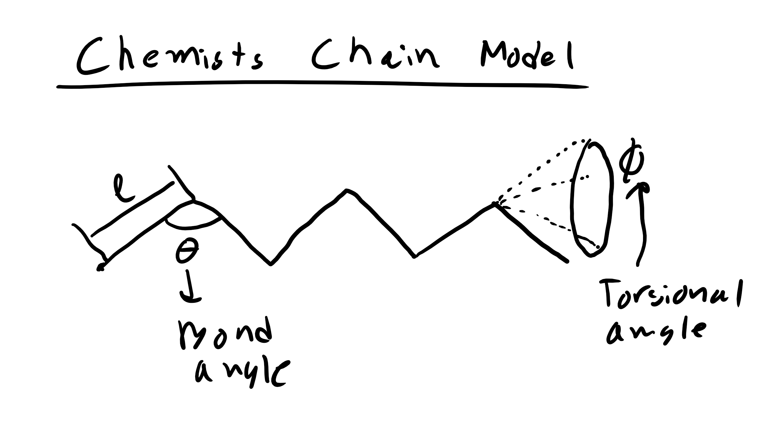
Let’s figure derive where these new values come from starting with going back to the matrix that we developed in the FJC model. So in the Chemist’s Model we assume that we have a fixed bond angle θ, makes sense thinking of polyethylene. Now the dot product of monomer i and i + 1 will be

\begin{equation}
\vec{l_{i}} \cdot \vec{l_{i+m}} = l^{2} (-\cos \theta)^m
\end{equation}

where m is an integer denoting the number of monomers away from monomer i, the θ keeps getting multiplied because of the projection of the the bond onto the next neighbor. You can see this model schematically here

Now we can adjust our previous matrix and get

\[
\langle\vec{r}_i \cdot \vec{r}_j \rangle =
\left[ {\begin{array}{ccccc}
l^2 & l^2(-\cos \theta) & l^2(\cos \theta)^2 & \ldots & l^2(- \cos \theta)^{n-1} \\
l^2(-\cos \theta) & l^2 & \ldots \\
\vdots & & & \ddots \\ \\
l^2 (- \cos \theta)^{n-1} & \ldots & & & l^2 \\
\end{array} } \right]
\]

And once you sum this matrix we find that

\begin{equation}
\langle r^2 \rangle = nl^2 \bigg (\frac{1-\cos \theta}{1+\cos\theta}\bigg )
\end{equation}

This factor of \(\frac{1- \cos \theta}{1+ \cos \theta}\) is

\begin{equation}
C_{\infty} = \frac{1- \cos \theta}{1+ \cos \theta}
\end{equation}

so now we get that

\begin{equation}
\langle r^2 \rangle = n l^2 C_{\infty}
\end{equation}

where C_∞ is the Flory characteristic ratio can be thought of as a measure of the stiffness of your monomer unit or how hard it is to rotate. You can look up this ratio for a number of different polymers and we should know that for C-C bonds θ = 109.5^o. Much more on Flory to come.

8.3.1 Rotational Isomeric States

Now this is an improvement but we have missed something very important and it is related to our discussion of conformers vs. isomers. We have previously briefly mentioned that there are certain molecules with different isomeric states, i.e. same chemical formula but distinct structures that can’t be related via rotation around a bond. A conformer or conformational isomer can be related different structures via rotations around a single bond and these different rotational states are called rotational isomeric states (RIS). Additionally these different states will each have different potential energies and thus we will find these different RIS states according to the weighted probabilities determined by the rotational potential V (ϕ). There are energy states where the bulky methyl groups overlap with either a hydrogen or another methyl group. Then we have our lower energy conformation as seen denoted by gauche ± and the lowest energy being the trans conformation. I wanted to illustrate this example because we did not treat this case in our derivation of the Chemist’s chain model so wee need to take this into account. Luckily we can do so using a very similar train of logic as we did above but instead of simply just using a fixed \(\cos \theta\)we need to take an ensemble average of the RIS angles based on the number of microstates for each angle so we will use

\begin{equation}
\langle \cos \phi \rangle = \frac{\int \cos \phi V(\phi) d \phi}{\int V(\phi)d \phi}
\end{equation}

and we eventually end up with (skipping full derivation as it is very very very extremely difficult)

\begin{equation}
\langle r^2 \rangle = nl^2 \bigg [ \bigg (\frac{1- \cos \theta}{1+ \cos \theta}\bigg) \bigg (\frac{1+ \langle \cos \phi \rangle}{1- \langle\cos \phi \rangle} \bigg) \bigg]
\end{equation}

And now we have our new and improved Flory Characteristic Ratio C_∞ which is

\begin{equation}
C_{\infty} = \bigg (\frac{1- \cos \theta}{1+ \cos \theta}\bigg) \bigg (\frac{1+ \langle \cos \phi \rangle}{1- \langle\cos \phi \rangle} \bigg)
\end{equation}

This derivation is beyond the scope of this course but you can look it up in Statistical Mechanics of Chain Molecules if you are interested, which is Flory’s text again much more Flory to come. Also some refer to this addition as the Hindered Rotation model.

Let’s take a moment here to stop to appreciate what we have just done. By taking into account bong angles and rotations we get fairly accurate values of C_∞ compared to experimental measurements and usually this value varies between 1-20. It’s important to note that C_∞ must always be at least 1 and this implies that the FJC/ideal chain is the most coiled conformation. This makes sense because by restricting these bond rotations we are inherently expanding our polymer chain, leading to a more elongated polymer. However our work is not finished yet. We have taken into account bond angles and bond rotation

but what else must we consider? Well does this model make any distinction between polymers that might have a large or bulky side chain? No! For these polymers with large bulky side chains we should expect that C_∞ should increase as the rotations are more difficult due to steric interactions.

So the increase is not due bonding interactions but due to excluded volume effects.

8.3.2 Excluded Volume

In order to capture these intramolecular steric interactions between monomers we have to talk about a somewhat initially obtuse concept of excluded volume. Excluded volume is the concept that monomers have some volume around them that other molecules can’t cross or move into this sphere. This takes care of the FJC ability of the chain to self-cross. These excluded volume interactions usually occur between monomers far apart on the polymer chain (because they must cross and intersect) and as you might imagine again like the bond angles and rotation this excluded volume effect will increase the \(\langle r^2 \rangle\) of the polymer chain.

Now this may still be a bit obtuse but you can visualize this excluded volume as a hard, impenetrable sphere that surround a given molecule or monomer. The size of the sphere must reflect the structure of the monomer. So a monomer, like polystyrene with a large bulky phenyl group will have a larger excluded volume than polyethylene with it’s hydrogen groups and no side chain. This excluded volume interaction will also depend on the interactions of the monomer with solvent interactions. If the monomer doesn’t like to interact with the solvent then the polymer will want to coil and collapse to avoid these interactions and thus the excluded volume will decreases and vice versa.

Remember that the solvent is the majority component and solute is the minority component.

8.4 Effect of Solvent on Polymer Chain MSD

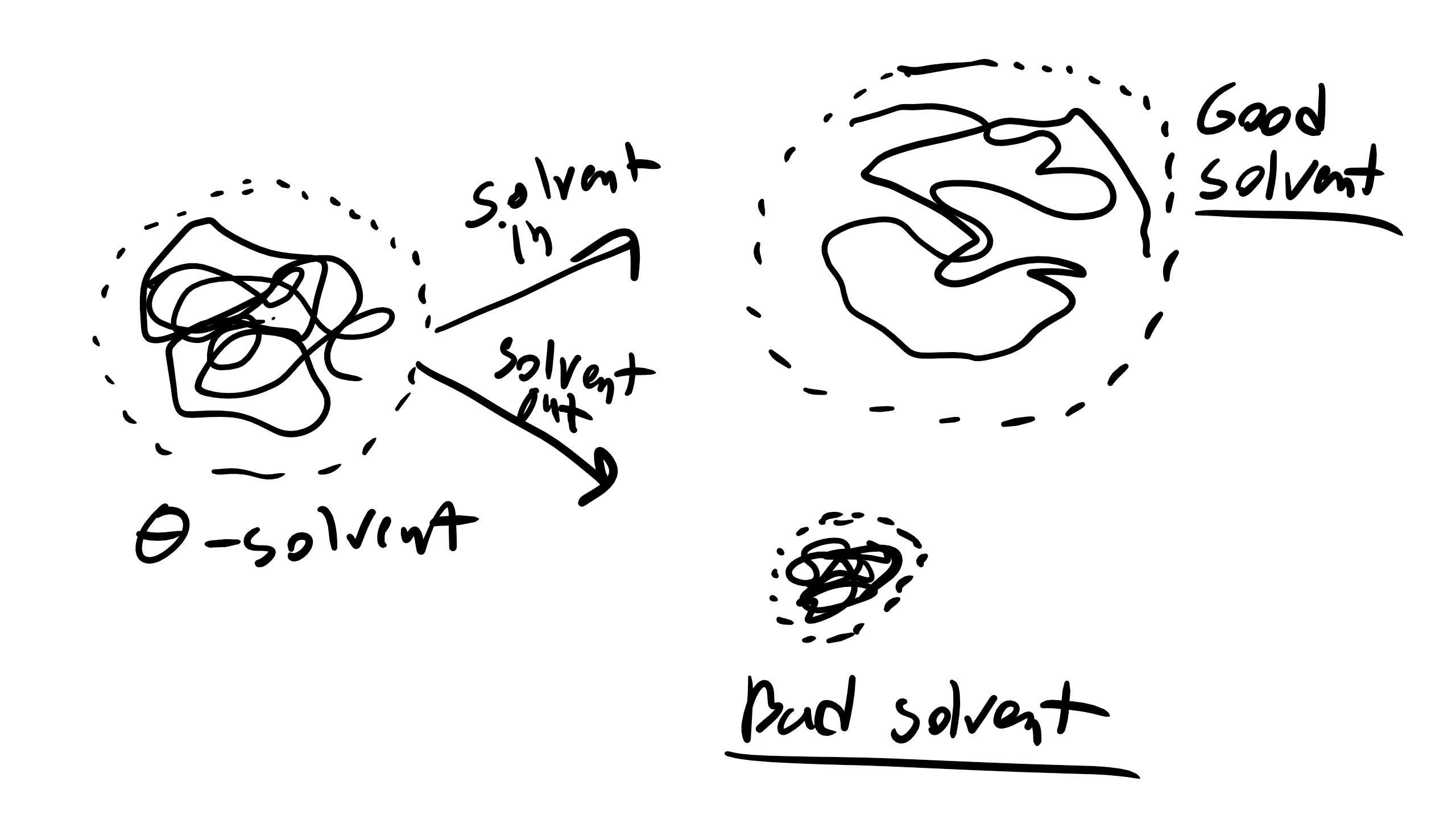
Speaking of solvent effect...as we mentioned in our Polymerization lecture there are times when the polymer is immersed in some type of solvent (i.e. water, alcohol, organic solvent, etc.). This solvent can have serious consequences on the dimension of our polymer chain. In good solvents, i.e. solvents were the polymer likes to interact with the solvent (favorable enthalpic intermolecular interactions), the polymer will extend in order to maximize the number of interactions between monomer and solvent. Conversely, if we are dealing with a bad solvent then the polymer doesn’t want to interact with the solvent and the polymer chain will fold in on itself and coil in order to minimize interactions with the solvent and the end-to-end distance will decrease. In the FJC/Ideal model we are in a very special condition with regards to solvent in that we are in a θ condition and thus in a theta solvent. In this condition you can imagine that upon mixing a polymer chain and a solvent the enthalpy of mixing is 0 just like an ideal solution. Alternatively you can imagine that excluded volume of the polymer chain does not change upon adding a θ solvent.

The parameter that we use to quantify the effect of solvent quality is measured via a factor \(\alpha\). Luckily \(\alpha\) is a fairly simple quantity to measure and is simply the ratio of the MSD end-to-end distance of the real chain in solution vs the chain in a θ solvent

\begin{equation}
\alpha^2 = \frac{\langle r^2 \rangle}{\langle r^2 \rangle_{\theta}}
\end{equation}

where \(\langle r^2 \rangle_{\theta}\) is the MSD of the chain in a θ solvent. So let’s define some values of \(\alpha^2\).

What will be the value of \(\alpha^2\) in a good solvent?

Well \(\alpha^2 >1\) for a good solvent.

What about a bad solvent? \(\alpha^2<1\) for a bad solvent What about a θ solvent? \(\alpha =1\) for a θ solvent

We will be talking much more about enthalpic interactions when we discuss Flory and whether enthalpic interactions are good/favorable and whether they are bad/poor/unfavorable interactions. We will talk about monomer-monomer interactions (ϵ_m−m), monomersolvent interactions (ϵ_m−s), and solvent-solvent (ϵ_s−s) interactions. Remember from the thermodynamic lecture that we always want lower or negative energies so for a good solvent ϵ_m−s should be the lowest energetic interaction and for bad solvent ϵ_m−s should be larger. Much more on this when we get to Flory.

So to quickly summarize

1. Mathematician’s Ideal Random Walk/Ideal Chain Model \(\langle r^2 \rangle =nl^2\)

• Assumes freely jointed chain, no bond angles, polymer can cross itself, no RIS states, steric interactions, or solvent/excluded volume interactions. Captures behavior of θ solvent and melt state fairly well.

2. Chemist’s Chain Model In Solution and Melt \(\langle r^2 \rangle = n l^2 C_\infty \alpha^2\)

• \(\theta\) Solvent or Melt \(\langle r^2 \rangle \approx nl^2\)

• Good Solvent \(\langle r^2 \rangle \approx n^\frac{6}{5}\)

• Poor Solvent \(\langle r^2 \rangle \approx n^{2/3}\)

• Takes into account preferred bond angles, steric interactions, RIS states, solvent, and excluded volume interactions.

8.9 Non-Crystalline/Amorphous Polymers:

Now that we have exhausted our discussion of semi-crystalline polymers we can move on to discussing non-crystalline/amorphous polymers which are polymers that do not undergo a melting transition but instead a glass transition when the temperature is lowered. These polymers then form amorphous but solid structures that lack the long range orientational and translational order of crystals.

8.9.1 Short Range and Long Range Order

Non-crystalline materials are characterized as having short-range order (SRO) but not long range orientational or long range translational order (LRO). This means that the probability of locating another atom within some distance r is more probable at certain short distances of r than at long distances, where the probability essentially becomes constant. Short-range order (SRO) arises because atoms prefer to pack together is characteristic of liquids in general due to a combination of bonding interactions and weak non-specific bonding. In polymers, SRO is due to local chemistry (such as polymer connectivity), excluded volume and the restricted conformational states due to the finite rotations of intramolecular covalent bonds. Long-range order arises in crystalline solids where the presence of translational symmetry (i.e. a well-defined unit cell) is due to highly specific, strong binding interactions (covalent bonds) or a strong non-specific intermolecular bonding. Polymers that exhibit short-range order but not long-range order are called amorphous; non-crystalline polymers are amorphous at all temperatures, while semi-crystalline polymers exhibit both amorphous regions and crystalline regions.

8.9.2 Glass Transition Temperature:

We have just discussed how non-crystalline amorphous polymers can be distinguished from semicrystalline polymers based on the presence of long range order. However, another critical parameter that is utilized to distinguish/describe amorphous polymers is the glass transition temperature (\T_g]). Typically, non-crystalline polymers can be broadly classified as either rubbery or glassy, both of which exist as highly interpenetrated/entangled Gaussian coils at relatively high temperatures above the glass transition temperature. When we say interpenetrated, the physical picture is of polymer coils that overlap with each other such that separate coils intertwine with each other. In this highly interpenetrated state, without solvent, the polymer acts as if it is unperturbed - that is, in the melt state the polymer is at the θ condition, and can be treated as an ideal chain. You can think of melt polymers as essentially feeling some pressure due to surrounding polymers that overcomes excluded volume effects, yielding an ideal state. The ideal nature of polymers in the melt make them much easier to think about theoretically.

The glass transition temperature is the temperature at which a polymer transitions from its fluid-like state to a glassy state. When we say a glass, we mean a material with only short-range order but lacking the translational fluctuations associated with liquids. Hence it is like a solid, but with randomly positioned atoms rather than ordered ones as we expect in a crystal. We can identify the physical origin of the glass transition temperature in two different ways - first, you can think of increasing the temperature from below the glass transition, or you can think of decreasing the temperature from above the glass transition temperature. In either case, the glass transition is a competition between the available thermal energy kT and the strength of intermolecular bonds ϵ_ij.

If we think of increasing temperature, then the glass transition temperature is the point at which thermal energy is sufficient to break local intermolecular bonds, enabling fluidlike motions - that is, the point where kT > ϵ_ij. If we think of decreasing temperature, then the glass transition temperature is the point at which the viscosity of the polymer essentially becomes infinite, eliminating molecular motion. In either case, the key property of a glass is that the rearrangement of atoms is hindered, limiting the ability of the system to relax to equilibrium when a stress/perturbation is applied. This is intimately related to the concept of a characteristic relaxation time which we will take a quick aside right now to discuss.

8.9.3 Relaxation Time τ^∗

The physical properties of amorphous polymers (and materials in general) are influenced by τ^∗, the characteristic relaxation time of the polymer, and how large this relaxation time is relative to a relevant experimental time (or the interaction time) t. The relaxation time is essentially a measure of how long it takes for a material to return to equilibrium after the application of some perturbation. The ratio between the relaxation time and experimental time is called the Deborah number - i.e. \(De = \frac{\tau^*}{t}\). It is easiest to think of the importance of the relaxation time in terms of known material behavior.

Let’s consider as an example a system consisting of some material in a container such that the material is magically attached to the container walls. We impose a perturbation on the system consisting of moving the walls of the container apart such that the material in the container is deformed/stretched. First consider the case that the relaxation time of a material is much smaller than the experimental time, such that τ^∗ << t and De << 1. Because the relaxation time is so much lower than the experimental time, the material effectively relaxes instantaneously to the new system dimensions as the perturbation is applied; in other words, the system adjusts to the new constraint by relaxing to equilibrium immediately. Physically, we could imagine this as the material rearranging its constituent molecules to instantaneously fill the new volume of the container - we would say that the material flows, and call the material in the container a liquid.

Now consider the opposite case, where the relaxation time is much greater than the experimental time such that τ^∗ >> t and De >> 1. Now when we adjust the walls of the container, the material effectively never relaxes to equilibrium as the perturbation occurs, instead being driven very far from equilibrium into a high energy state. In our physical example, we would imagine the material in the container being stretched but being unable to adjust the positions of its atoms because the relaxation time is so long, so that the material instead builds up a large amount of strain energy; we would consider this an elastic response and call the material an elastic solid. Note that the only distinction we are drawing here between the liquid and solid case is the experimental time - this implies that if we apply a stress/strain to a solid and wait long enough, it would appear to flow like a liquid (in the case of crystalline solids this would be due to the gradual movement of defects throughout the material to change the solid dimensions). In an intermediate regime where the relaxation time is roughly the same as the experimental time, the material will exhibit behavior consistent with both viscous liquids and elastic solids; we call these materials viscoelastic and will discuss their properties much more in future lectures.

We can gain some understanding of relaxation times from the molecular structure of a given material. For example, for small molecules like water, the relatively free motion of water due to its small size would lead to a small relaxation time, and hence water is only solid at low temperatures. Polymers tend to exhibit a longer relaxation time due to the connectivity monomers, requiring collective motion to adjust to a perturbation. As we will discuss shortly, at lower temperatures the energetic cost for this motion is too great to allow the polymer to flow, leading to glassy behavior. We might also imagine, then, that polymers with more rigid backbones have longer relaxation times due to the lessened flexibility of the chain.

Characterizing a polymer as a rubber, liquid, or solid (glass) is impossible without further information on the overall environment, as the response of the polymer depends on the time scales involved. We will also see that the relaxation time in polymers is a function of temperature, yielding many of the characteristic mechanical properties which we will discuss in future lectures. To wrap up if the molecular motion is slow/hindered, the relaxation time of the polymer is very long and thus the polymer exhibits solid-like behavior.

8.9.4 Back to Glass Transition Temperatures:

A key point about the glass transition temperature is that it is not strictly a thermodynamic transition. The melting temperature, for example, results because there is some specific temperature for materials where the free energy of the liquid phase becomes lower than the free energy of the solid phase, leading to melting behavior (and more specifically there is an abrupt change in thermodynamic quantities reflecting a first-order phase transition). Hence, the melting point is thermodynamic in nature, resulting from the competition between the higher entropy liquid phase and lower enthalpy solid phase. The glass transition is not strictly thermodynamic, as a glass is not a stable thermodynamic phase but rather a kinetically-trapped phase resulting from the large energy barriers faced by a glass when it must adjust to a perturbation.

The glass transition thus reflects the kinetics and time scale of a system and as such the transition temperature is not easily defined - in fact, the exact measurement depends on cooling rate and typically a range of glass transition temperatures are reported for specific samples.

8.9.5 T_g and Chemical Structure of Monomers:

Trends in T_g can be explained by looking at the chemical structure of monomers due to the influence of monomer structure on both chain flexibility and free volume. Recall that T_g is determined by the onset of long range cooperative molecular motion, meaning the motion of 10-30 connected chain monomers at once. The cooperative motion requires both sufficient thermal energy to induce the movement of these monomers and sufficient free volume for the monomers to move into. Both of these requirements are influenced by monomer structure. There are essentially 3 elements of monomer structure that can influence these motions:

1. Chain interactions - energetic interactions between monomers

2. Ease of rotation about main chain bonds - whether there is significant steric hindrance to rotation

3. Amount of free volume available - how densely the monomers pack

We can think of polymers as essentially divided into their backbone and sidechains coming from that backbone. In polymers with flexible backbones, like polyethylene (lots of C-C single bonds) and PDMS (Si-O bonds, which are flexible due to the 4 electrons on the oxygen atoms in place of hydrogens), the hindrance to rotation is low and hence less thermal energy is necessary to induce molecular motion, leading to a low T_g. On the other hand, polymers with phenyl molecules along the backbone (e.g. polycarbonate) tend to have a much higher T_g, since the bulky phenyl constituent greatly increases the amount of energy necessary for rotation (i.e. the rigidity). Note that we can generally relate C_∞ to the rigidity of a backbone, and hence expect T_g to increase with C_∞.

Similarly, large bulky sidechains, such as phenyl groups, also oppose rotation due to steric hindrance, and in addition decrease the amount of free volume available since they occupy a greater excluded volume, leading to a higher glass transition temperature. Finally, intermolecular interactions, such as hydrogen bonds or ionic interactions, which are typically seen between sidechains, will tend to greatly increase the glass transition temperature since thermal energy will also have to break these bonds to induce rotation. The lecture notes provide some examples of polymers, sidechains, and the related T_g. The main principles to keep in mind are that chain flexibility allows easier cooperative movement of monomers, decreasing the T_g, and increased free volume around the chain backbone lowers the barrier to cooperative movement and hence decreases the T_g.

We can also relate these observations back to the idea of crystallinity, as well, as the factors that influence the glass transition temperature will also influence the ability of polymers to crystallize. In fact, there is a correlation between T_g and T_m for semi-crystalline polymers - typically T_g is about 0.5 to 0.8 T_m in Kelvin.

8.10 XRD Analysis

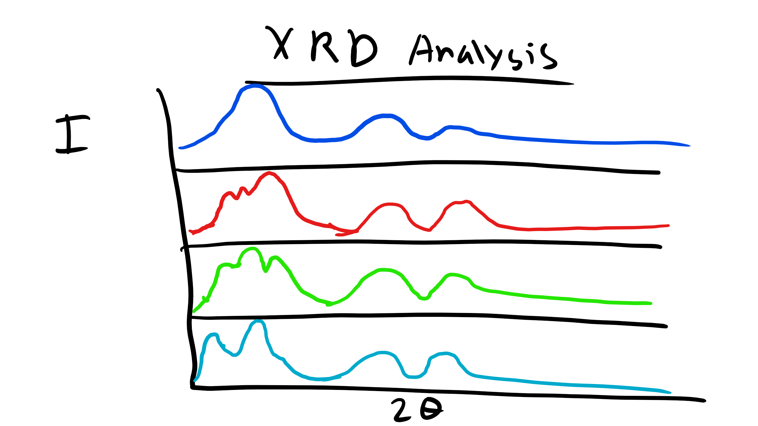
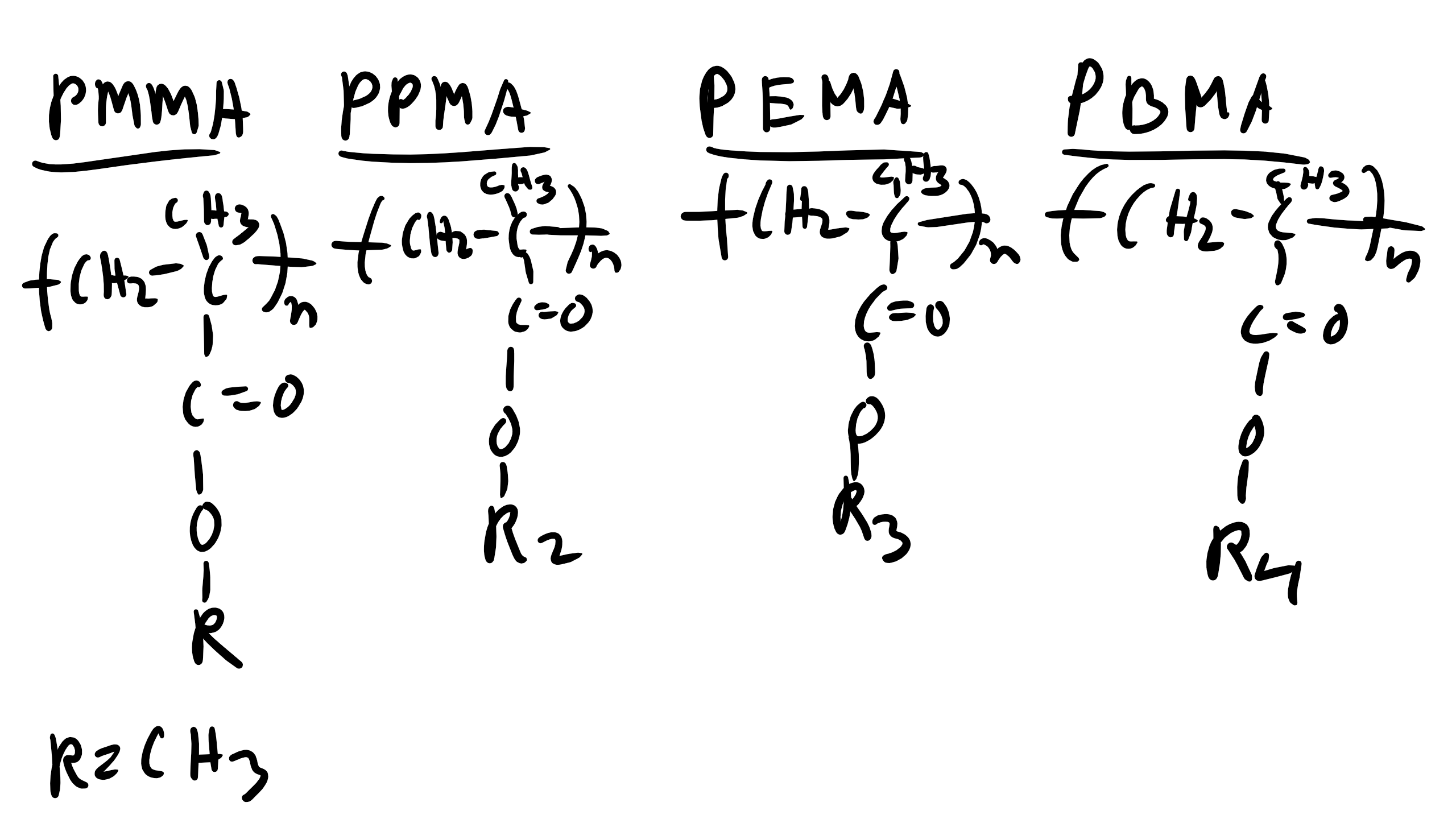
We have talked about XRD analysis and have done our XRD lab which included a polymer. We know that the peaks observed in the diffractogram will be more broad than that for metals due to the lack of long range translational and orientational order for polymers. However, we can obtain some key information from XRD analysis of polymers to allow us to deduce some information about the structure of polymers and how they might be arranged. Let’s take for example the case of the family of polymethacrylates, specifically PMMA, PPMA, PEMA, and PBMA.

When we examine the XRD profile of these polymers we can see that there are some XRD peaks that do not shift for the entire family of polymers. Additionally, the peaks that appear to be consistent between the family are all located at large Bragg angles (2θ). At lower Bragg angles there appears a considerable amount of peak shifting and perhaps even some creation or destruction of peaks in the XRD curve. How can we explain what is happening here?

Well again remember that we observe peaks in the XRD curves when there is constructive interference which occurs when at that particularly incident angle there is some local order perhaps even long-range order of some type.

We also know from Bragg’s law that the Bragg Angle \(\theta \propto \frac{1}{d}\). So the characteristic distance where this local order appears is inversely proportional to the incident angle. Let’s think about the structure of these polymers at very short distances like the C-C bond distance or the distance between the methyl groups. This distance will not change depending on the polymer we are looking at in this family. These small distances correspond to large angles and so this explains why the peaks are conserved for the different polymers.

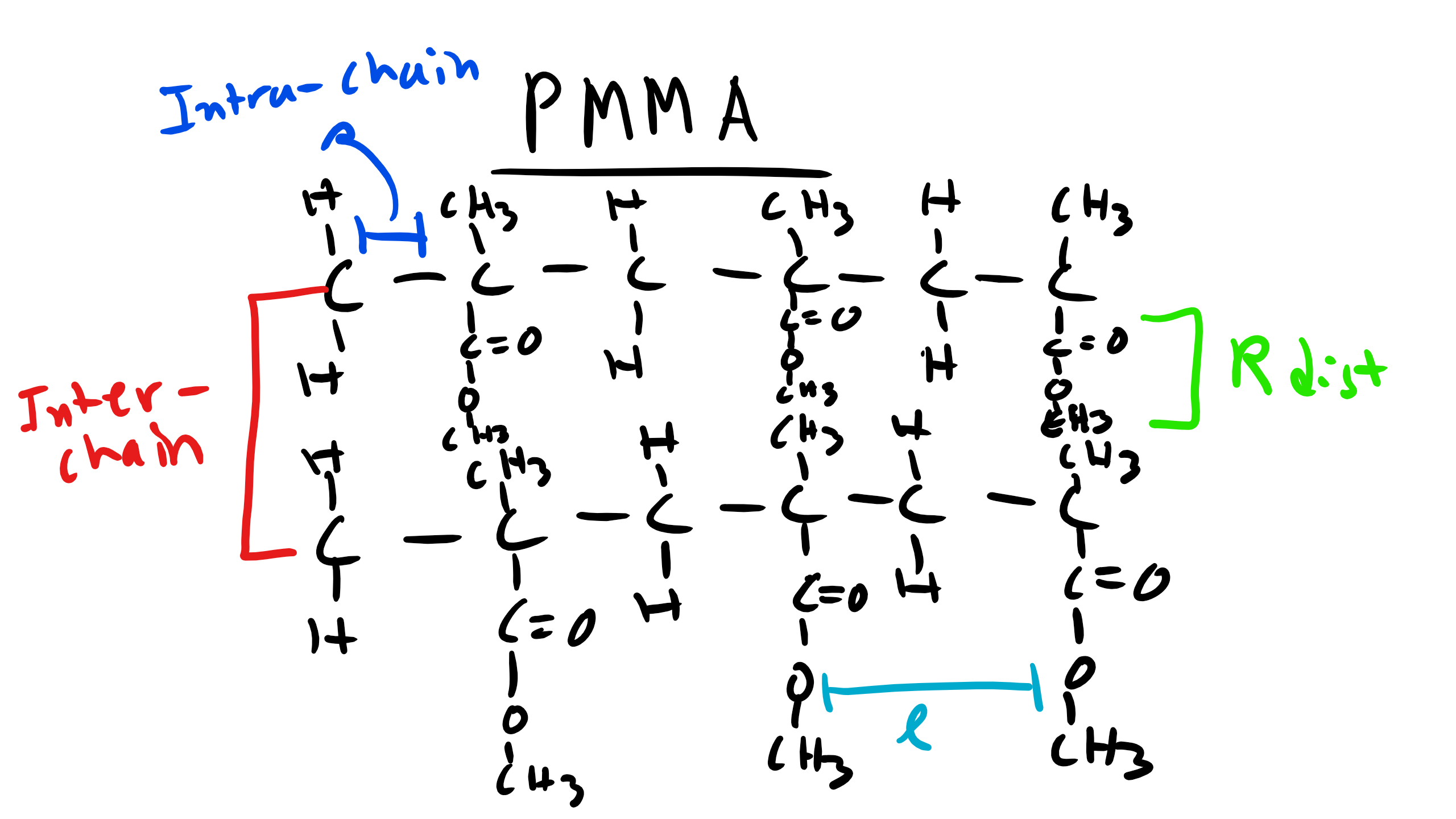
Now what is happening for the other polymers. Well there are other characteristic distances for these polymers. For example the distance from the chain backbone to the end of the R functional group. Or even the inter-chain distance within the polymer. These distances will change depending on whether the polymer is PMMA, PBMA, etc. If the distance changes there will be a corresponding shift in the location of the peaks. And we see that on average as the side group R increases in length for these polymers the peaks tend to shift to the left which is consistent from what we know about diffraction! This is critical information as it gives us a schematic of the structural characteristics of an unknown polymer chain.

8.11 DSC Analysis:

Differential Scanning Calorimetry (DSC) is a thermal analysis technique useful for measuring thermodynamic properties of materials such as specific heat, melting point, boiling point, glass transition temperature (in amorphous/semi-crystalline materials), heat of fusion, reaction kinetics, etc. The technique measures the temperature and the heat flow, corresponding to the thermal performance of materials, both as a function of time and temperature.

Typically a DSC will utilize a heat flux type system in which the differential heat flux between a reference (e.g. sealed empty aluminum pan) and a sample (encapsulated in a similar pan) is measured. The reference and the sample pans are placed on separate, but identical, stages on a thermoelectric sensor platform surrounded by a furnace. As the temperature of the furnace is changed (usually by heating at a linear rate), heat is transferred to the sample and reference through the thermoelectric platform. The heat flow difference between the sample and the reference is then measured by measuring the temperature difference between them by using thermocouples attached to the respective stages. The DSC provides qualitative and quantitative information on endothermic heat absorption (e.g. melting) and exothermic heat release (e.g. solidification or fusion). These processes display sharp deviation from the steady state thermal profile, and exhibit peaks and valleys in a DSC thermogram (heat flow vs. temperature profile). The latent heat of melting or fusion can then be obtained from the area enclosed within the peak or valley.

DSC analysis is an extremely critical and useful tool in characterizing the thermodynamic quantities of polymer, specifically in identifying T_g and T_m as well as determining if a polymer is amorphous or crystalline.

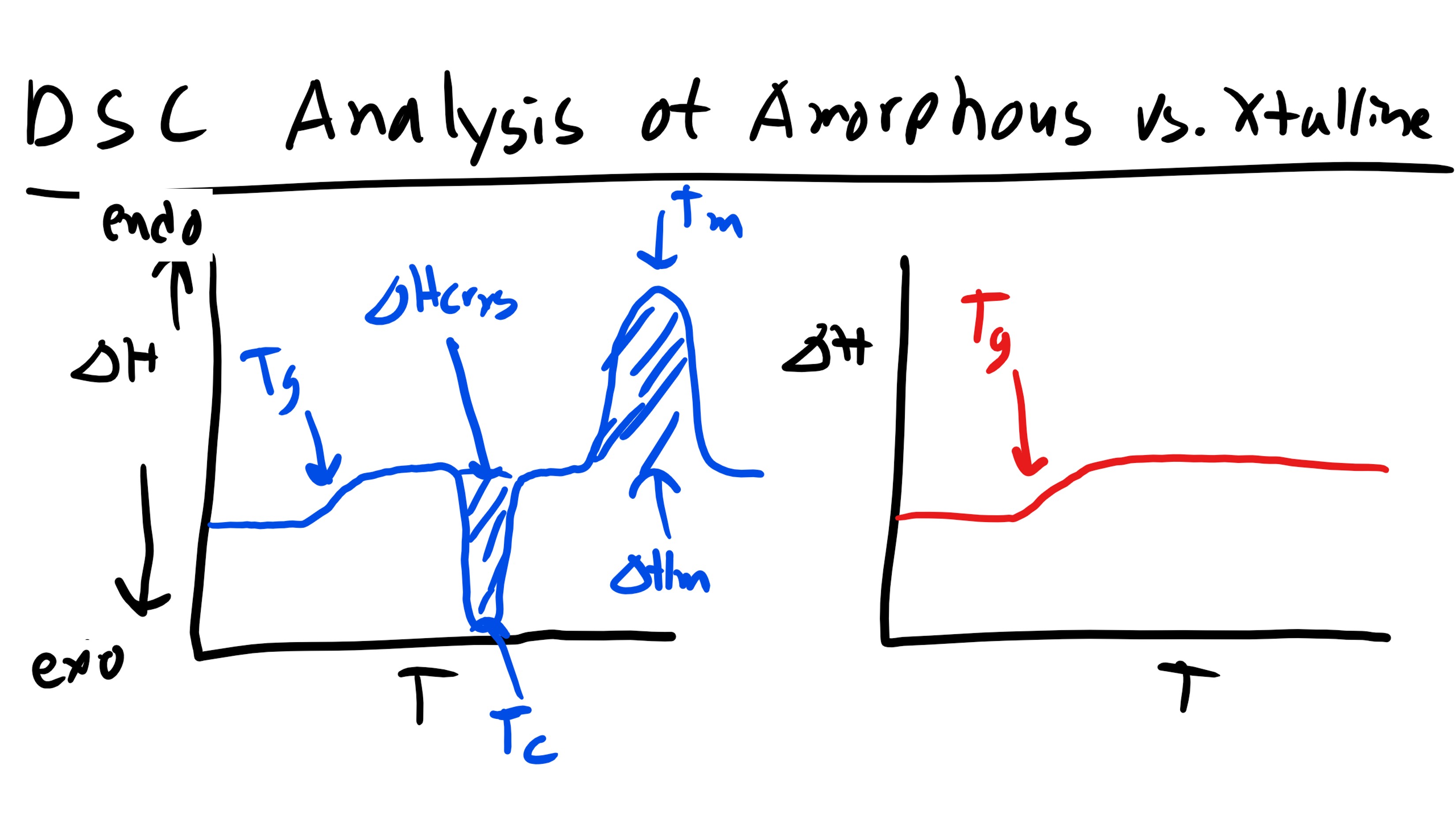
As you can see below if we are working a polymer that is semi-crystalline we can typically observe 2 peaks in the DSC curve as well as a change in the slope of the curve of heat flow vs temperature. Let’s take this analysis step by step. If we remember back to Materials Science we know that a first order phase transition will result in a discontinuity in the first order derivative of the free energy as a function of temperature (at the temperature of the transition). Whereas second order transitions will exhibit a discontinuity in the second derivative of the free energy and will only exhibit a change in slope for the first derivative as a function of temperature. Now the plot that we are looking at is heat flow vs temperature which is essentially \(\Delta H\) vs T so we are looking at a plot of the first derivative of free energy.

Now the first feature that we come across (increasing in temperature) is a change in slope. Well we know this must be a second order transition. Additionally we know that this transition occurred at fairly low temperatures. Since our sample is a polymer this transition most likely signifies the glass transition temperature, T_g. This should make sense as we know the T_g is a second order transition. Now the next feature that we see is an exothermic peak. Well we know that this peak indicates a first order transition and if this is an exothermic reaction this should signify some solidification or re-crystallization, T_c. This might at first seem counter-intuitive, why would increasing temperature cause the polymer to crystallize? Well it is because as we increase temperature we increase the mobility of the previously glass amorphous regions. With this increased mobility there is a higher likelihood of encountering other chains the enthalpic interactions accessed here might favor the formation of crystalline regions. This curve might not show up in every polymer. The last peak is an endothermic one and we will recognize this as the melting point, T_m. Now remember this does not break the carbon-carbon backbone bonds but instead the secondary intermolecular interactions.

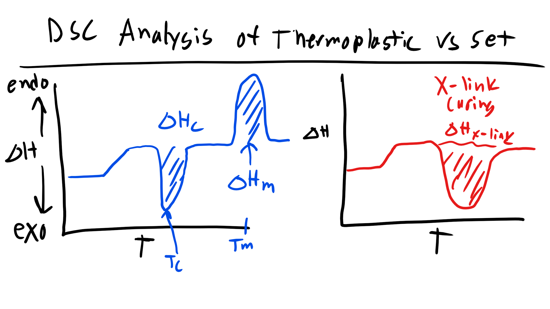
How would this curve change for a purely amorphous polymer? Well we would simply see a change in the slope to indicate the glass transition and the would be it. Now what if you had a thermoset polymer which has to cure and form crosslinks. Well, we would see a T_g as this is still a polymer. Now would you see a melting temperature? No a thermoset does not undergo melting due to the permanent crosslinks! They would exhibit an exothermic peak that would indicate the energy required to cure/crosslink the polymer!