Superparamagnetism

Superparamagnetism is a form of magnetism exhibited by small ferromagnetic or ferrimagnetic nanoparticles. At sizes of less than a hundred nanometers, the nanoparticles are single-domain particles, allowing the magnetization of the nanoparticles to be approximated as one giant magnetic moment by summing the individual magnetic moments of each constituent atom. This approximation is called the “macro-spin approximation.” When the nanoparticles are small enough, the energy barriers for magnetization reversal, which are proportional to grain volume, are relatively low compared to thermal energy. With enough thermal energy, their magnetization can flip direction randomly over short periods of time and the time between two flips in direction is called the Neel relaxation time. The superparamagnetic state refers to how the average magnetization of the nanoparticles averages to zero when no external magnetic field is applied and the measurement time for the magnetization of the nanoparticles is greater than the Neel relaxation time. With an external magnetic field applied, the nanoparticles are magnetized like paramagnets, but with much greater susceptibility.

While any ferromagnetic or ferromagnetic material can exhibit paramagnetic behavior, the difference is that this usually occurs above the Curie temperature whereas in superparamagnets, this occurs below the Curie temperature.

Properties of Superparamagnets

Neel Relaxation Time

Nanoparticles typically have magnetic anisotropy, meaning they have a preferred direction for magnetization alignment. As a result, the magnetic moment usually has only two stable, antiparallel orientations separated by an energy barrier. The two stable orientations are defined as along the nanoparticle's "easy axis." Thermal energy causes the nanoparticles to randomly flip the direction of their magnetization and the average time between two flips, or the Neel Relaxation time τ_N, is given by the Neel-Arrhenius equation:

\[ \tau_N = \tau_0 \exp \left(\frac {KV}{k_BT}\right) \]

where

• \(\tau_0\) is the attempt time or attempt period, and is a characteristic length of time of the material. It usually ranges from 10^-9 to 10^-12 seconds.
• \(K\) is the magnetic anisotropy energy density of the nanoparticle and \(V\) is the volume. \(KV\) gives the energy barrier for the magnetization flip to overcome.
• \(k_B\) is the Boltzmann constant.
• \(T\) is the temperature.

Blocking Temperature

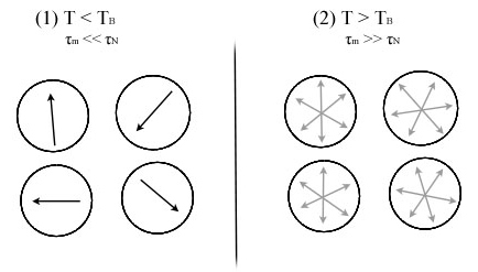
Another factor in observing superparamagnetism is the measurement time τ_m. When the measurement time is much less than the Neel relaxation time (τ_m << τ_N), a blocked state occurs in which the measured magnetization is just the instantaneous magnetization at the beginning of the measurement because there was no direction flip. In this state, the nanomaterials behave like a normal paramagnet but with a much higher susceptibility. When the measurement time is much greater than the Neel relaxation time (τ_m >> τ_N), this results in the superparamagnetic state in which the net moment is zero due to the fluctuations in magnetization. These two states are illustrated in Figure 1 below. The blocking temperature,T_B, is the temperature between the blocked and superparamagnetic states, or the temperature at which τ_m = τ_N. It can be calculated by the following equation:

\[ T_B = \frac{KV}{k_B \ln \left(\frac{\tau_m}{\tau_0}\right)} \]

Some typical measurement times for different types of measurements are as follows:

• DC magnetization: 100 seconds
• AC susceptibility: 10^-1 to 10^-5 seconds
• Mössbauer spectroscopy: 10^-7 to 10 ^-9 seconds.

Figure \(\PageIndex{1}\): Case 1 illustrates the blocked state at temperatures lower than the blocking temperature in which the magnetic moment of each particle is well-defined. Case 2 shows the superparamagnetic state at temperatures above the blocking temperature. In this state, the magnetization direction constantly flips directions, resulting in an observed net moment of zero.

Magnetization Curves

When an external magnetic field is applied to superparamagnetic particles, the particles have a net magnetization because the magnetic moments of the particles will begin to align with the applied field. Assuming that all the particles are of similar size, there are two possible cases for the net magnetization and the corresponding susceptibility, depending on the temperature T.

• When \( T_B < T < KV/10k_B \), the easy axes are parallel to the external field. The net magnetization and susceptibility are approximately defined as:

\( M(H) = n\mu\tanh(\frac{\mu_0H\mu}{k_BT}) \)

\( \chi = \frac{n\mu_0\mu^2}{k_BT} \)

• When \( T > KV/k_B \), the easy axes orientation no longer affects the magnetization and the equations for net magnetization and susceptibility are now:

\( M(H) = n\mu L(\frac{\mu_0H\mu}{k_BT}) \)

\( \chi = \frac{n\mu_0\mu^2}{3k_BT} \)

In these equations, the variables are defined as follows:

• \( n \) is the density of nanoparticles
• \( \mu \) is the magnetic moment of the nanoparticle
• \(\mu_0 \) is the magnetic constant or the magnetic permeability of vacuum
• \( L \) refers to the Langevin function, which is defined as \( L(x) = 1/\tanh(x) - 1/x \)

Size Dependence

As mentioned in the introduction, superparamagnetivity occurs due to the small size of the particles. In Figure 2 below, the magnetization of paramagnetic, ferromagnetic and superparamagnetic materials in response to an external magnetic field.

Figure 2: The magnetization curves (plots of magnetization M vs. applied field H) for paramagnetic, ferromagnetic, and superparamagnetic (when T > T_B) materials.

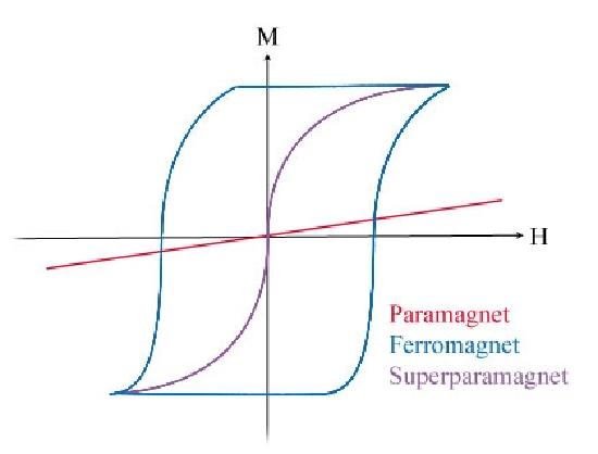
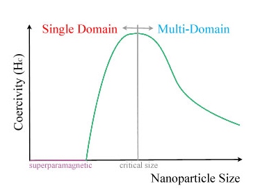
As shown in the above figure, the ferromagnetic response has a hysteresis loop. When ferromagnetic particles increase in size, the magnetic moment increases, which in turn increases the magnetization and allows the magnetization to reach its saturation, or maximum, value quicker. This translates to a thinner hysteresis loop. Conversely, decreasing the particle size will widen the hysteresis loop until a certain nanoparticle size, called the critical size. Once this size is reached, the hysteresis loop begins to narrow with decreasing size until the superparamagnetic size threshold is reached. When the nanoparticles reach superparamagnetic sizes, response curve retains the sigmoidal shape of a ferromagnetic response but loses the loop. Figure 3 below shows this pattern in a plot of coercivity, or the intensity of the applied magnetic field to yield a zero magnetization, against nanoparticle size.

Figure 3: This plot shows that decreasing the nanoparticle size increases the coercivity H_C until the critical size. Between the critical size and superparamagnetic threshold, decreasing the nanoparticle size decreases the coercivity. Once the coercivity hits zero, the nanoparticle is superparamagnetic.

Limitations and Applications

Hard Drives

The superparamagnetic limit refers how superparamagnetism limits the storage capacity of hard drive disks (HDDs) by setting a minimum size for the magnetic grains used.

In an HDD, data, or bits, is stored on platters of concentric tracks as a sequence of magnetization direction changes. Reading these platters refers to translating the magnetization into a voltage and writing is just the reverse process. Within a single bit cell are many magnetic grains. In order to decrease the transition noise, the size of the magnetic grains must be decreased. However, when the grain sizes are too small, they become superparamagnetic. Magnetic grains retain data by holding the magnetization given to them during the writing process but if the grains are too small, thermal fluctuations will cause the magnetizations to change.

Magnetic Resonance Imaging

One biomedical application of superparamagnets is in contrast enhancement agents for magnetic resonance imaging (MRI).

MRIs work by applying an external magnetic field to the body to magnetize particles in the body and then measuring the relaxation time of the tissues. By attaching the nanoparticles to cell or compound, the relaxation times can be shortened,and greater contrast can be achieved since the type of tissue can determine how well the nanoparticles are absorbed.

Drug Delivery

Superparamagnetic nanoparticles are used in drug delivery by being attached to a drug and having a magnetic force control its path. Once the drug has reached the intended location, it can be released from the carrier by enzymes or physiological changes in the body.

Ferrofluids

Ferrofluids are fluids in which evenly dispersed magnetic nanograins are suspended in a liquid. Ferrofluids have another mechanism aside from Neel relaxation that changes the directions of the particles' magnetic moments called Brownian relaxation, which cause the grains to physically spin due to collisions with nearby particles. When ferrofluids are placed in a strong vertical magnetic field, they experience normal-field instability. By trying to align their magnetic moments with the field lines of the external field and field lines of their neighbors, the magnetic particles move in lines along the external magnetic field lines, resulting in spikes forming on the liquid surface.

Applications for ferrofluids include heat transfer, such as in a loudspeaker for cooling the voice coil, and damping, by increasing the viscosity of liquid flow due to an effect called the magnetorheological effect.

Questions

1. What is the energy barrier (in eV) for a superparamagnetic material with a characteristic time of 5 x 10^-10 seconds and a relaxation time of 1 second at 300 K?
2. In the case of question 1, what is the blocking temperature of the material if the measurement time is 100 seconds?
3. How does the magnetization curve of a superparamagnet compare to those of a paramagnet and a ferromagnet?

Answers

1. The energy barrier can be calculated using the equation for the Neel relaxation time, which states:

\( \tau_N = \tau_0 exp(\frac {KV}{k_BT}) \)

and the problem defines the variables as follows:

\(\tau_N = 1 s\)

\(\tau_0 = 5*10^{-10} s \)

\(T = 300 K\)

\(k_B = 8.62*10^{-5} eV/K\)

First, solve for the energy barrier, or \(KV\), from the Neel relaxation equation.

\( \tau_N = \tau_0 exp(\frac {KV}{k_BT}) \)

\( \tau_N/ \tau_0= exp(\frac {KV}{k_BT}) \)

\( \ln(\tau_N/ \tau_0) = \frac {KV}{k_BT} \)

\(k_BT\ln(\tau_N/\tau_0) = KV \)

Now, plug in the values from earlier into this new equation:

\(KV = 8.62*10^{-5}*300*\ln(\frac{1}{5*10^{-10}}) \)

\( KV = 0.554 eV\)

2. To calculate the blocking temperature, use the blocking temperature equation:

\( T_B = \frac{KV}{k_Bln(\frac{\tau_m}{\tau_0})} \)

and use the values from the previous problem as well as the new information to set the variables as:

\(\tau_m = 100 s \)

\(\tau_0 = 5*10^{-10} s \)

\(KV = 0.554 eV \)

\(k_B = 8.62*10^{-5} eV/K\)

Plugging these values directly into the equation results in:

\( T_B = \frac{0.554}{8.62*10^{-5}*ln(\frac{100}{5*10^{-10}} )} \)

\( T_B = 247 K\)

3. The magnetization curves of a superparamagnet and a paramagnet both have positive susceptibility and zero coercivity. However, the susceptibility is much greater for a superparamagnet than a normal paramagnet. For the ferromagnet and the superparamagnet, the magnetization curves both take on a sigmoidal shape but the superparamagnetic curve does not have a hysteresis loop and has a zero coercivity.

References

1. Wikipedia. Superparamagnetism. Retrieved on Dec. 7, 2015 from https://en.Wikipedia.org/wiki/Superparamagnetism
2. Benz, Manuel. Superparamagnetism: Theory and Application. 2012.
3. Bowles, Julie, Mike Jackson, Amy Chen, and Peter Solheid. The Quarterly. 3rd ed. Vol. 19. Minneapolis, MN: IRM, 2009. Web. 7 Dec. 2015.
4. Petracic, O. Superparamagnetic nanoparticle ensembles. Germany.
5. Marolt, Miha. Superparamagnetic materials. Slovenia. 2014.
6. Wikipedia. Coercivity. Retrieved on Dec. 8, 2015 from https://en.Wikipedia.org/wiki/Coercivity

Contributors and Attributions

• Tina Li (University of California, Davis)