
25.1: Model Problem- n = 2 Spring-Mass System in Equilibrium
- Page ID
- 55698

Description
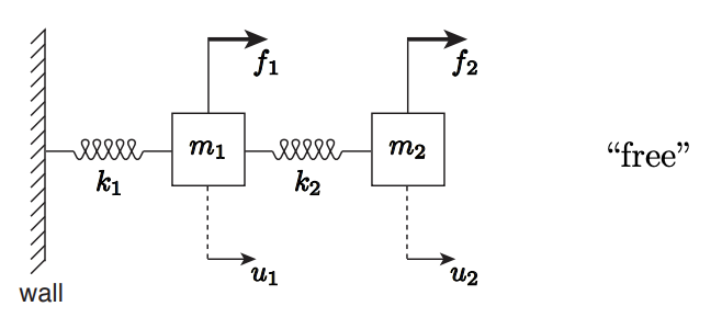
We will introduce here a simple spring-mass system, shown in Figure \(\underline{25.1}\), which we will use throughout this chapter to illustrate various concepts associated with linear systems and associated solution techniques. Mass 1 has mass \(m_{1}\) and is connected to a stationary wall by a spring with stiffness \(k_{1}\). Mass 2 has mass of \(m_{2}\) and is connected to the mass \(m_{1}\) by a spring with stiffness \(k_{2}\).
We denote the displacements of mass 1 and mass 2 by \(u_{1}\) and \(u_{2}\), respectively: positive values correspond to displacement away from the wall; we choose our reference such that in the absence of applied forces - the springs unstretched \(-u_{1}=u_{2}=0\). We next introduce (steady) forces \(f_{1}\) and \(f_{2}\) on mass 1 and mass 2, respectively; positive values correspond to force away from the wall. We are interested in predicting the equilibrium displacements of the two masses, \(u_{1}\) and \(u_{2}\), for prescribed forces \(f_{1}\) and \(f_{2}\).
We note that while all real systems are inherently dissipative and therefore are characterized not just by springs and masses but also dampers, the dampers (or damping coefficients) do not affect the system at equilibrium - since \(d / d t\) vanishes in the steady state - and hence for equilibrium considerations we may neglect losses. Of course, it is damping which ensures that the system ultimately achieves a stationary (time-independent) equilibrium. \({ }_{-}^{1}\)
\({ }^{1}\) In some rather special cases - which we will study later in this chapter - the equilibrium displacement is indeed affected by the initial conditions and damping. This special case in fact helps us better understand the mathematical aspects of systems of linear equations.


We now derive the equations which must be satisfied by the displacements \(u_{1}\) and \(u_{2}\) at equilibrium. We first consider the forces on mass 1, as shown in Figure 25.2. Note we apply here Hooke’s law - a constitutive relation - to relate the force in the spring to the compression or extension of the spring. In equilibrium the sum of the forces on mass 1 - the applied forces and the forces due to the spring - must sum to zero, which yields \[f_{1}-k_{1} u_{1}+k_{2}\left(u_{2}-u_{1}\right)=0 .\] (More generally, for a system not in equilibrium, the right-hand side would be \(m_{1} \ddot{u}_{1}\) rather than zero.) A similar identification of the forces on mass 2, shown in Figure \(25.3\), yields for force balance \[f_{2}-k_{2}\left(u_{2}-u_{1}\right)=0 .\] This completes the physical statement of the problem.
Mathematically, our equations correspond to a system of \(n=2\) linear equations, more precisely, 2 equations in 2 unknowns: \[\begin{aligned} \left(k_{1}+k_{2}\right) u_{1}-k_{2} u_{2} &=f_{1}, \\ -k_{2} u_{1}+k_{2} u_{2} &=f_{2} . \end{aligned}\] Here \(u_{1}\) and \(u_{2}\) are unknown, and are placed on the left-hand side of the equations, and \(f_{1}\) and \(f_{2}\) are known, and placed on the right-hand side of the equations. In this chapter we ask several questions about this linear system - and more generally about linear systems of \(n\) equations in \(n\) unknowns. First, existence: when do the equations have a solution? Second, uniqueness: if a solution exists, is it unique? Although these issues appear quite theoretical in most cases the mathematical subtleties are in fact informed by physical (modeling) considerations. In later chapters in this unit we will ask a more obviously practical issue: how do we solve systems of linear equations efficiently?
But to achieve these many goals we must put these equations in matrix form in order to best take advantage of both the theoretical and practical machinery of linear algebra. As we have already addressed the translation of sets of equations into corresponding matrix form in Unit III (related to overdetermined systems), our treatment here shall be brief.
We write our two equations in two unknowns as \(K u=f\), where \(K\) is a \(2 \times 2\) matrix, \(u=\left(u_{1} u_{2}\right)^{\mathrm{T}}\) is a \(2 \times 1\) vector, and \(f=\left(\begin{array}{lll}f_{1} & f_{2}\end{array}\right)^{\mathrm{T}}\) is a \(2 \times 1\) vector. The elements of \(K\) are the coefficients of the equations \(\underline{(25.1)}\) and \((\underline{25.2})\) :
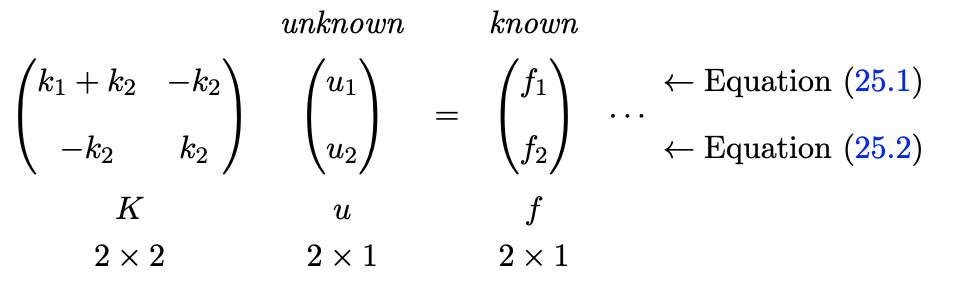
We briefly note the connection between equations (25.3) and (25.1). We first note that \(K u=F\) implies equality of the two vectors \(K u\) and \(F\) and hence equality of each component of \(K u\) and \(F\). The first component of the vector \(K u\), from the row interpretation of matrix multiplication, \({ }_{-}\) is given by \(\left(k_{1}+k_{2}\right) u_{1}-k_{2} u_{2}\); the first component of the vector \(F\) is of course \(f_{1}\). We thus conclude that \((K u)_{1}=f_{1}\) correctly produces equation (25.1). A similar argument reveals that the \((K u)_{2}=f_{2}\) correctly produces equation (25.2).
Property
We recall that a real \(n \times n\) matrix \(A\) is Symmetric Positive Definite (SPD) if \(A\) is symmetric \[A^{\mathrm{T}}=A ,\] and \(A\) is positive definite \[v^{\mathrm{T}} A v>0 \text { for any } v \neq 0 .\] Note in equation (25.5) that \(A v\) is an \(n \times 1\) vector and hence \(v^{\mathrm{T}}(A v)\) is a scalar - a real number. Note also that the positive definite property (25.5) implies that if \(v^{\mathrm{T}} A v=0\) then \(v\) must be the zero vector. There is also a connection to eigenvalues: symmetry implies real eigenvalues, and positive definite implies strictly positive eigenvalues (and in particular, no zero eigenvalues).
There are many implications of the SPD property, all very pleasant. In the context of the current unit, an SPD matrix ensures positive eigenvalues which in turn will ensure existence and uniqueness of a solution - which is the topic of the next section. Furthermore, an SPD matrix ensures stability of the Gaussian elimination process - the latter is the topic in the following chapters. We also note that, although in this unit we shall focus on direct solvers, SPD matrices also offer advantages in the context of iterative solvers: the very simple and efficient conjugate gradient method can be applied (only to) SPD matrices. The SPD property is also the basis of minimization principles which serve in a variety of contexts. Finally, we note that the SPD property is often, though not always, tied to a natural physical notion of energy.
We shall illustrate the SPD property for our simple \(2 \times 2\) matrix \(K\) associated with our spring system. In particular, we now again consider our system of two springs and two masses but now we introduce an arbitrary imposed displacement vector \(v=\left(\begin{array}{ll}v_{1} & v_{2}\end{array}\right)^{\mathrm{T}}\), as shown in Figure 25.4. In this case our matrix \(A\) is given by \(K\) where
\({ }^{2}\) In many, but not all, cases it is more intuitive to develop matrix equations from the row interpretation of matrix multiplication; however, as we shall see, the column interpretation of matrix multiplication can be very important from the theoretical perspective.

We can then form the scalar \(v^{\mathrm{T}} K v\) as \[\begin{aligned} v^{\mathrm{T}} K v &=v^{\mathrm{T}} \underbrace{\left(\begin{array}{cc} k_{1}+k_{2} & -k_{2} \\ -k_{2} & k_{2} \end{array}\right)\left(\begin{array}{c} v_{1} \\ v_{2} \end{array}\right)}_{K v} \\ &=\left(\begin{array}{ll} v_{1} & v_{2} \end{array}\right) \underbrace{}_{\left.\begin{array}{cc} \left(k_{1}+k_{2}\right) v_{1} & -k_{2} v_{2} \\ -k_{2} v_{1} & k_{2} v_{2} \end{array}\right)} \\ &=v_{1}^{2}\left(k_{1}+k_{2}\right)-v_{1} v_{2} k_{2}-v_{2} v_{1} k_{2}+v_{2}^{2} k_{2} \\ &=v_{1}^{2} k_{1}+\left(v_{1}^{2}-2 v_{1} v_{2}+v_{2}^{2}\right) k_{2} \\ &=k_{1} v_{1}^{2}+k_{2}\left(v_{1}-v_{2}\right)^{2} . \end{aligned}\] We now inspect this result.
In particular, we may conclude that, under our assumption of positive spring constants, \(v^{\mathrm{T}} K v \geq\) 0 . Furthermore, \(v^{\mathrm{T}} K v\) can only be zero if \(v_{1}=0\) and \(v_{1}=v_{2}\), which in turn implies that \(v^{\mathrm{T}} K v\) can only be zero if both \(v_{1}\) and \(v_{2}\) are zero \(-v=0\). We thus see that \(K\) is SPD: \(v^{\mathrm{T}} K v>0\) unless \(v=0\) (in which case of course \(v^{\mathrm{T}} K v=0\) ). Note that if either \(k_{1}=0\) or \(k_{2}=0\) then the matrix is not SPD: for example, if \(k_{1}=0\) then \(v^{\mathrm{T}} K v=0\) for any \(v=\left(\begin{array}{cc}c & c\end{array}\right)^{\mathrm{T}}, c\) a real constant; similarly, if \(k_{2}=0\), then \(v^{\mathrm{T}} K v=0\) for any \(v=\left(\begin{array}{ll}0 & c\end{array}\right)^{\mathrm{T}}, c\) a real constant.
We can in this case readily identify the connection between the SPD property and energy. In particular, for our spring system, the potential energy in the spring system is simply \(\frac{1}{2} v^{\mathrm{T}} K v\) :
\(\mathrm{PE}\) (potential/elastic energy) \(=\) \[\underbrace{\frac{1}{2} k_{1} v_{1}^{2}}_{\begin{array}{c} \text { energy in } \\ \text { spring } 1 \end{array}}+\underbrace{\frac{1}{2} k_{2}\left(v_{2}-v_{1}\right)^{2}}_{\begin{array}{c} \text { energy in } \\ \text { spring } 2 \end{array}}=\frac{1}{2} v^{\mathrm{T}} A v>0 \quad(\text { unless } v=0)\] where of course the final conclusion is only valid for strictly positive spring constants. Finally, we note that many MechE systems yield models which in turn may be described by SPD systems: structures (trusses, ...); linear elasticity; heat conduction; flow in porous media (Darcy’s Law); Stokes (or creeping) flow of an incompressible fluid. (This latter is somewhat complicated by the incompressibility constraint.) All these systems are very important in practice and indeed ubiquitous in engineering analysis and design. However, it is also essential to note that many other very important MechE phenomena and systems - for example, forced convection heat transfer, non-creeping fluid flow, and acoustics - do not yield models which may be described by SPD matrices.