25.2: Existence and Uniqueness- n = 2

Problem Statement

We shall now consider the existence and uniqueness of solutions to a general system of \((n=) 2\) equations in ( \(n=) 2\) unknowns. We first introduce a matrix \(A\) and vector \(f\) as \[\begin{aligned} &2 \times 2 \text { matrix } \quad A=\left(\begin{array}{ll} A_{11} & A_{12} \\ A_{21} & A_{22} \end{array}\right) \\ &2 \times 1 \text { vector } \quad f=\left(\begin{array}{l} f_{1} \\ f_{2} \end{array}\right) \end{aligned}\] our equation for the \(2 \times 1\) unknown vector \(u\) can then be written as \[\left.A u=f, \quad \text { or } \quad\left(\begin{array}{cc} A_{11} & A_{12} \\ A_{21} & A_{22} \end{array}\right)\left(\begin{array}{l} u_{1} \\ u_{2} \end{array}\right)=\left(\begin{array}{c} f_{1} \\ f_{2} \end{array}\right), \quad \text { or } \quad \begin{array}{lll} A_{11} u_{1}+A_{12} u_{2}= & f_{1} \\ A_{21} u_{1}+A_{22} u_{2}=f_{2} \end{array}\right\} .\] Note these three expressions are equivalent statements proceeding from the more abstract to the more concrete. We now consider existence and uniqueness; we shall subsequently interpret our general conclusions in terms of our simple \(n=2\) spring-mass system.

View

We first consider the row view, similar to the row view of matrix multiplication. In this perspective we consider our solution vector \(u=\left(\begin{array}{ll}u_{1} & u_{2}\end{array}\right)^{\mathrm{T}}\) as a point \(\left(u_{1}, u_{2}\right)\) in the two dimensional Cartesian plane; a general point in the plane is denoted by \(\left(v_{1}, v_{2}\right)\) corresponding to a vector \(\left(v_{1} \quad v_{2}\right)^{\mathrm{T}}\). In particular, \(u\) is the particular point in the plane which lies both on the straight line described by the first equation, \((A v)_{1}=f_{1}\), denoted ’eqn1’ and shown in Figure \(25.5\) in blue, and on the straight line described by the second equation, \((A v)_{2}=f_{2}\), denoted ’eqn2’ and shown in Figure \(25.5\) in green.

We directly observe three possibilities, familiar from any first course in algebra; these three cases are shown in Figure 25.6. In case (i), the two lines are of different slope and there is clearly one and only one intersection: the solution thus exists and is furthermore unique. In case (ii) the two lines are of the same slope and furthermore coincident: a solution exists, but it is not unique - in fact, there are an infinity of solutions. This case corresponds to the situation in which the two equations in fact contain identical information. In case (iii) the two lines are of the same slope but not coincident: no solution exists (and hence we need not consider uniqueness). This case corresponds to the situation in which the two equations contain inconsistent information.

Figure 25.5: Row perspective: \(u\) is the intersection of two straight lines.

Figure 25.6: Three possibilities for existence and uniqueness; row interpretation.

Figure 25.7: Parallelogram construction for the case in case in which a unique solution exists.

We see that the condition for (both) existence and uniqueness is that the slopes of ’eqn1’ and ’eqn2’ must be different, or \(A_{11} / A_{12} \neq A_{21} / A_{22}\), or \(A_{11} A_{22}-A_{12} A_{21} \neq 0\). We recognize the latter as the more familiar condition \(\operatorname{det}(A) \neq 0\). In summary, if \(\operatorname{det}(A) \neq 0\) then our matrix \(A\) is nonsingular and the system \(A u=f\) has a unique solution; if \(\operatorname{det}(A) \neq 0\) then our matrix \(A\) is singular and either our system has an infinity of solutions or no solution, depending on \(f\). (In actual practice the determinant condition is not particularly practical computationally, and serves primarily as a convenient "by hand" check for very small systems.) We recall that a non-singular matrix \(A\) has an inverse \(A^{-1}\) and hence in case \((i)\) we can write \(u=A^{-1} f\); we presented this equation earlier under the assumption that \(A\) is non-singular - now we have provided the condition under which this assumption is true.

Column View

We next consider the column view, analogous to the column view of matrix multiplication. In particular, we recall from the column view of matrix-vector multiplication that we can express \(A u\) as \[A u=\left(\begin{array}{ll} A_{11} & A_{12} \\ A_{21} & A_{22} \end{array}\right)\left(\begin{array}{l} u_{1} \\ u_{2} \end{array}\right)=\underbrace{\left(\begin{array}{c} A_{11} \\ A_{21} \end{array}\right)}_{p^{1}} u_{1}+\underbrace{\left(\begin{array}{l} A_{12} \\ A_{22} \end{array}\right)}_{p^{2}},\] where \(p^{1}\) and \(p^{2}\) are the first and second column of \(A\), respectively. Our system of equations can thus be expressed as \[A u=f \quad \Leftrightarrow \quad p^{1} u_{1}+p^{2} u_{2}=f .\] Thus the question of existence and uniqueness can be stated alternatively: is there a (unique?) combination, \(u\), of columns \(p^{1}\) and \(p^{2}\) which yields \(f\) ?

We start by answering this question pictorially in terms of the familiar parallelogram construction of the sum of two vectors. To recall the parallelogram construction, we first consider in detail the case shown in Figure 25.7. We see that in the instance depicted in Figure \(25.7\) there is clearly a unique solution: we choose \(u_{1}\) such that \(f-u_{1} p^{1}\) is parallel to \(p^{2}\) (there is clearly only one such value of \(u_{1}\) ); we then choose \(u_{2}\) such that \(u_{2} p^{2}=f-u_{1} p^{1}\).

We can then identify, in terms of the parallelogram construction, three possibilities; these three cases are shown in Figure 25.8. Here case \((i)\) is the case already discussed in Figure 25.7: a unique solution exists. In both cases (ii) and (iii) we note that \[p^{2}=\gamma p^{1} \quad \text { or } \quad p^{2}-\gamma p^{1}=0\left(p^{1} \text { and } p^{2} \text { are linearly dependent }\right)\] for some \(\gamma\), where \(\gamma\) is a scalar; in other words, \(p^{1}\) and \(p^{2}\) are colinear - point in the same direction to within a sign (though \(p^{1}\) and \(p^{2}\) may of course be of different magnitude). We now discuss these two cases in more detail.

Figure 25.8: Three possibilities for existence and uniqueness; the column perspective.

In case \((i i), p^{1}\) and \(p^{2}\) are colinear but \(f\) also is colinear with \(p^{1}\) (and \(p^{2}\) ) - say \(f=\beta p^{1}\) for some scalar \(\beta\). We can thus write \[\begin{aligned} f &=p^{1} \cdot \beta+p^{2} \cdot 0 \\ &=\left(\begin{array}{ll} p^{1} & p^{2} \end{array}\right)\left(\begin{array}{l} \beta \\ 0 \end{array}\right) \\ &=\left(\begin{array}{ll} A_{11} & A_{12} \\ A_{21} & A_{22} \end{array}\right) \underbrace{\left(\begin{array}{l} \beta_{0} \\ 0 \end{array}\right)}_{u^{*}} \\ &=A u^{*}, \end{aligned}\] and hence \(u^{*}\) is a solution. However, we also know that \(-\gamma p^{1}+p^{2}=0\), and hence \[\begin{aligned} 0 &=p^{1} \cdot(-\gamma)+p^{2} \cdot(1) \\ &=\left(\begin{array}{ll} p^{1} & p^{2} \end{array}\right)\left(\begin{array}{c} -\gamma \\ 1 \end{array}\right) \\ &=\left(\begin{array}{cc} A_{11} & A_{12} \\ A_{21} & A_{22} \end{array}\right)\left(\begin{array}{c} -\gamma \\ 1 \end{array}\right) \\ &=A\left(\begin{array}{c} -\gamma \\ 1 \end{array}\right) \end{aligned}\] Thus, for any \(\alpha\), \[u=\underbrace{u^{*}+\alpha\left(\begin{array}{c} -\gamma \\ 1 \end{array}\right)}_{\text {infinity of solutions }}\] satisfies \(A u=f\), since \[\begin{aligned} A\left(u^{*}+\alpha\left(\begin{array}{c} -\gamma \\ 1 \end{array}\right)\right) &=A u^{*}+A\left(\alpha\left(\begin{array}{c} -\gamma \\ 1 \end{array}\right)\right) \\ &=A u^{*}+\alpha A\left(\begin{array}{c} -\gamma \\ 1 \end{array}\right) \\ &=f+\alpha \cdot 0 \\ &=f \end{aligned}\] This demonstrates that in case \((i i)\) there are an infinity of solutions parametrized by the arbitrary constant \(\alpha\).

Finally, we consider case (iii). In this case it is clear from our parallelogram construction that for no choice of \(v_{1}\) will \(f-v_{1} p^{1}\) be parallel to \(p^{2}\), and hence for no choice of \(v_{2}\) can we form \(f-v_{1} p^{1}\) as \(v_{2} p^{2}\). Put differently, a linear combination of two colinear vectors \(p^{1}\) and \(p^{2}\) can not combine to form a vector perpendicular to both \(p^{1}\) and \(p^{2}\). Thus no solution exists.

Note that the vector \((-\gamma 1)^{\mathrm{T}}\) is an eigenvector of \(A\) corresponding to a zero eigenvalue. \({ }^{3}\) By definition the matrix \(A\) has no effect on an eigenvector associated with a zero eigenvalue, and it is for this reason that if we have one solution to \(A u=f\) then we may add to this solution any multiple - here \(\alpha\) - of the zero-eigenvalue eigenvector to obtain yet another solution. More generally a matrix \(A\) is non-singular if and only if it has no zero eigenvalues; in that case - case \((i)-\) the inverse exists and we may write \(u=A^{-1} f\). On the other hand, if \(A\) has any zero eigenvalues then \(A\) is singular and the inverse does not exist; in that case \(A u=f\) may have either many solutions or no solutions, depending on \(f\). From our discussion of SPD systems we also note that \(A\) SPD is a sufficient (but not necessary) condition for the existence of the inverse of \(A\).

Tale of Two Springs

We now interpret our results for existence and uniqueness for a mechanical system - our two springs and masses - to understand the connection between the model and the mathematics. We again consider our two masses and two springs, shown in Figure \(25.9\), governed by the system of equations \[A u=f \quad \text { for } \quad A=K \equiv\left(\begin{array}{cc} k_{1}+k_{2} & -k_{2} \\ -k_{2} & k_{2} \end{array}\right) \text {. }\] We analyze three different scenarios for the spring constants and forces, denoted (I), (II), and (III), which we will see correspond to cases (i), (ii), and (iii), respectively, as regards existence and uniqueness. We present first (I), then (III), and then (II), as this order is more physically intuitive.

(I) In scenario (I) we choose \(k_{1}=k_{2}=1\) (more physically we would take \(k_{1}=k_{2}=\bar{k}\) for some value of \(\bar{k}\) expressed in appropriate units - but our conclusions will be the same) and \(f_{1}=f_{2}=1\) (more physically we would take \(f_{1}=f_{2}=\bar{f}\) for some value of \(\bar{f}\) expressed in appropriate units - but our conclusions will be the same). In this case our matrix \(A\) and

\({ }^{3}\) All scalar multiples of this eigenvector define what is known as the right nullspace of \(A\).

Figure 25.9: System of equilibrium equations for two springs and two masses.

associated column vectors \(p^{1}\) and \(p^{2}\) take the form shown below. It is clear that \(p^{1}\) and \(p^{2}\) are not colinear and hence a unique solution exists for any \(f\). We are in case \((i)\). \[=\left(\begin{array}{rr} 2 & -1 \\ -1 & 1 \end{array}\right)\]

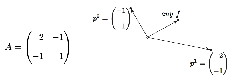
case \((i)\) : exists \(\mathfrak{\checkmark}\), unique \(\mathfrak{\checkmark}\)

(III) In scenario (III) we chose \(k_{1}=0, k_{2}=1\) and \(f_{1}=f_{2}=1\). In this case our vector \(f\) and matrix \(A\) and associated column vectors \(p^{1}\) and \(p^{2}\) take the form shown below. It is clear that a linear combination of \(p^{1}\) and \(p^{2}\) can not possibly represent \(f\) - and hence no solution exists. We are in case (iii).

case (\(iii\)): exists \(\boldsymbol{X}\), \(\cancel{unique}\)

We can readily identify the cause of the difficulty. For our particular choice of spring constants
in scenario (III) the first mass is no longer connected to the wall (since \(k_{1}=0\) ); thus our in scenario (III) the first mass is no longer connected to the wall (since \(k_{1}=0\) ); thus our spring system now appears as in Figure \(\frac{25.10}{}\). We see that there is a net force on our system (of two masses) - the net force is \(f_{1}+f_{2}=2 \neq 0-\) and hence it is clearly inconsistent to assume equilibrium. \({ }^{4}\) In even greater detail, we see that the equilibrium equations for each mass are inconsistent (note \(f_{\mathrm{spr}}=k_{2}\left(u_{2}-u_{1}\right)\) ) and hence we must replace the zeros on the right-hand sides with mass \(\times\) acceleration terms. At fault here is not the mathematics but rather the model provided for the physical system.

\({ }^{4}\) In contrast, in scenario (I), the wall provides the necessary reaction force in order to ensure equilibrium.

Figure 25.10: Scenario III

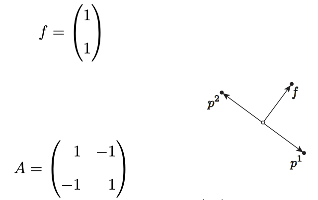
(II) In this scenario we choose \(k_{1}=0, k_{2}=1\) and \(f_{1}=1, f_{2}=-1\). In this case our vector \(f\) and matrix \(A\) and associated column vectors \(p^{1}\) and \(p^{2}\) take the form shown below. It is clear that a linear combination of \(p^{1}\) and \(p^{2}\) now can represent \(f\) - and in fact there are many possible combinations. We are in case (\(ii\)).

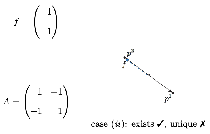
We can explicitly construct the family of solutions from the general procedure described earlier: \[\begin{aligned} p^{2} &==\underbrace{-1}_{\gamma} p^{1} \\ f &=\underbrace{-1}_{\beta} p^{1} \Rightarrow u^{*}=\left(\begin{array}{c} =-1 \\ 0= \end{array}\right) \\ u &=u^{*}+\alpha\left(\begin{array}{c} -\gamma \\ 1 \end{array}\right) \\ &=\left(\begin{array}{c} -1 \\ 0 \end{array}\right)+\alpha\left(\begin{array}{l} 1 \\ 1 \end{array}\right) \end{aligned}\] e stretched)

Figure 25.11: Scenario II. (Note on the left mass the \(f_{1}\) arrow indicates the direction of the force \(f_{1}=-1\), not the direction of positive force.)

for any \(\alpha\). Let us check the result explicitly: \[\begin{aligned} A\left(\left(\begin{array}{c} -1 \\ 0 \end{array}\right)+\left(\begin{array}{l} \alpha \\ \alpha \end{array}\right)\right) &=\left(\begin{array}{rr} 1 & -1 \\ -1 & 1 \end{array}\right)\left(\begin{array}{c} 1+\alpha \\ \alpha \end{array}\right) \\ &=\left(\begin{array}{c} (-1+\alpha)-\alpha \\ (1-\alpha)+\alpha \end{array}\right) \\ &=\left(\begin{array}{c} -1 \\ 1 \end{array}\right) \\ &=f \end{aligned}\] as desired. Note that the zero-eigenvalue eigenvector here is given by \(\left(\begin{array}{ll}-\gamma & 1\end{array}\right)^{\mathrm{T}}=\left(\begin{array}{ll}1 & 1\end{array}\right)^{\mathrm{T}}\) and corresponds to an equal (or translation) shift in both displacements, which we will now interpret physically.

In particular, we can readily identify the cause of the non-uniqueness. For our choice of spring constants in scenario (II) the first mass is no longer connected to the wall (since \(k_{1}=0\) ), just as in scenario (III). Thus our spring system now appears as in Figure \(25.11\). But unlike in scenario (III), in scenario (II) the net force on the system is zero \(-f_{1}\) and \(f_{2}\) point in opposite directions - and hence an equilibrium is possible. Furthermore, we see that each mass is in equilibrium for a spring force \(f_{\mathrm{spr}}=1\). Why then is there not a unique solution? Because to obtain \(f_{\mathrm{spr}}=1\) we may choose any displacements \(u\) such that \(u_{2}-u_{1}=1\) (for \(k_{2}=1\) ): the system is not anchored to wall - it just floats - and thus equilibrium is maintained if we shift (or translate) both masses by the same displacement (our eigenvector) such that the "stretch" remains invariant. This is illustrated in Figure 25.12, in which \(\alpha\) is the shift in displacement. Note \(\alpha\) is not determined by the equilibrium model; \(\alpha\) could be determined from a dynamical model and in particular would depend on the initial conditions and the

Figure 25.12: Scenario (II): non-uniqueness.

damping in the system.

We close this section by noting that for scenario (I) \(k_{1}>0\) and \(k_{2}>0\) and hence \(A(\equiv K)\) is SPD: thus \(A^{-1}\) exists and \(A u=f\) has a unique solution for any forces \(f\). In contrast, in scenarios (II) and (III), \(k_{1}=0\), and hence \(A\) is no longer SPD, and we are no longer guaranteed that \(A^{-1}\) exists - and indeed it does not exist. We also note that in scenario (III) the zero-eigenvalue eigenvector \(\left(\begin{array}{ll}1 & 1\end{array}\right)^{\mathrm{T}}\) is precisely the \(v\) which yields zero energy, and indeed a shift (or translation) of our unanchored spring system does not affect the energy in the spring.