
17.2: Centroids of Areas via Integration
- Page ID
- 55339

\( \newcommand{\vecs}[1]{\overset { \scriptstyle \rightharpoonup} {\mathbf{#1}} } \)
\( \newcommand{\vecd}[1]{\overset{-\!-\!\rightharpoonup}{\vphantom{a}\smash {#1}}} \)
\( \newcommand{\dsum}{\displaystyle\sum\limits} \)
\( \newcommand{\dint}{\displaystyle\int\limits} \)
\( \newcommand{\dlim}{\displaystyle\lim\limits} \)
\( \newcommand{\id}{\mathrm{id}}\) \( \newcommand{\Span}{\mathrm{span}}\)
( \newcommand{\kernel}{\mathrm{null}\,}\) \( \newcommand{\range}{\mathrm{range}\,}\)
\( \newcommand{\RealPart}{\mathrm{Re}}\) \( \newcommand{\ImaginaryPart}{\mathrm{Im}}\)
\( \newcommand{\Argument}{\mathrm{Arg}}\) \( \newcommand{\norm}[1]{\| #1 \|}\)
\( \newcommand{\inner}[2]{\langle #1, #2 \rangle}\)
\( \newcommand{\Span}{\mathrm{span}}\)
\( \newcommand{\id}{\mathrm{id}}\)
\( \newcommand{\Span}{\mathrm{span}}\)
\( \newcommand{\kernel}{\mathrm{null}\,}\)
\( \newcommand{\range}{\mathrm{range}\,}\)
\( \newcommand{\RealPart}{\mathrm{Re}}\)
\( \newcommand{\ImaginaryPart}{\mathrm{Im}}\)
\( \newcommand{\Argument}{\mathrm{Arg}}\)
\( \newcommand{\norm}[1]{\| #1 \|}\)
\( \newcommand{\inner}[2]{\langle #1, #2 \rangle}\)
\( \newcommand{\Span}{\mathrm{span}}\) \( \newcommand{\AA}{\unicode[.8,0]{x212B}}\)
\( \newcommand{\vectorA}[1]{\vec{#1}} % arrow\)
\( \newcommand{\vectorAt}[1]{\vec{\text{#1}}} % arrow\)
\( \newcommand{\vectorB}[1]{\overset { \scriptstyle \rightharpoonup} {\mathbf{#1}} } \)
\( \newcommand{\vectorC}[1]{\textbf{#1}} \)
\( \newcommand{\vectorD}[1]{\overrightarrow{#1}} \)
\( \newcommand{\vectorDt}[1]{\overrightarrow{\text{#1}}} \)
\( \newcommand{\vectE}[1]{\overset{-\!-\!\rightharpoonup}{\vphantom{a}\smash{\mathbf {#1}}}} \)
\( \newcommand{\vecs}[1]{\overset { \scriptstyle \rightharpoonup} {\mathbf{#1}} } \)
\(\newcommand{\longvect}{\overrightarrow}\)
\( \newcommand{\vecd}[1]{\overset{-\!-\!\rightharpoonup}{\vphantom{a}\smash {#1}}} \)
\(\newcommand{\avec}{\mathbf a}\) \(\newcommand{\bvec}{\mathbf b}\) \(\newcommand{\cvec}{\mathbf c}\) \(\newcommand{\dvec}{\mathbf d}\) \(\newcommand{\dtil}{\widetilde{\mathbf d}}\) \(\newcommand{\evec}{\mathbf e}\) \(\newcommand{\fvec}{\mathbf f}\) \(\newcommand{\nvec}{\mathbf n}\) \(\newcommand{\pvec}{\mathbf p}\) \(\newcommand{\qvec}{\mathbf q}\) \(\newcommand{\svec}{\mathbf s}\) \(\newcommand{\tvec}{\mathbf t}\) \(\newcommand{\uvec}{\mathbf u}\) \(\newcommand{\vvec}{\mathbf v}\) \(\newcommand{\wvec}{\mathbf w}\) \(\newcommand{\xvec}{\mathbf x}\) \(\newcommand{\yvec}{\mathbf y}\) \(\newcommand{\zvec}{\mathbf z}\) \(\newcommand{\rvec}{\mathbf r}\) \(\newcommand{\mvec}{\mathbf m}\) \(\newcommand{\zerovec}{\mathbf 0}\) \(\newcommand{\onevec}{\mathbf 1}\) \(\newcommand{\real}{\mathbb R}\) \(\newcommand{\twovec}[2]{\left[\begin{array}{r}#1 \\ #2 \end{array}\right]}\) \(\newcommand{\ctwovec}[2]{\left[\begin{array}{c}#1 \\ #2 \end{array}\right]}\) \(\newcommand{\threevec}[3]{\left[\begin{array}{r}#1 \\ #2 \\ #3 \end{array}\right]}\) \(\newcommand{\cthreevec}[3]{\left[\begin{array}{c}#1 \\ #2 \\ #3 \end{array}\right]}\) \(\newcommand{\fourvec}[4]{\left[\begin{array}{r}#1 \\ #2 \\ #3 \\ #4 \end{array}\right]}\) \(\newcommand{\cfourvec}[4]{\left[\begin{array}{c}#1 \\ #2 \\ #3 \\ #4 \end{array}\right]}\) \(\newcommand{\fivevec}[5]{\left[\begin{array}{r}#1 \\ #2 \\ #3 \\ #4 \\ #5 \\ \end{array}\right]}\) \(\newcommand{\cfivevec}[5]{\left[\begin{array}{c}#1 \\ #2 \\ #3 \\ #4 \\ #5 \\ \end{array}\right]}\) \(\newcommand{\mattwo}[4]{\left[\begin{array}{rr}#1 \amp #2 \\ #3 \amp #4 \\ \end{array}\right]}\) \(\newcommand{\laspan}[1]{\text{Span}\{#1\}}\) \(\newcommand{\bcal}{\cal B}\) \(\newcommand{\ccal}{\cal C}\) \(\newcommand{\scal}{\cal S}\) \(\newcommand{\wcal}{\cal W}\) \(\newcommand{\ecal}{\cal E}\) \(\newcommand{\coords}[2]{\left\{#1\right\}_{#2}}\) \(\newcommand{\gray}[1]{\color{gray}{#1}}\) \(\newcommand{\lgray}[1]{\color{lightgray}{#1}}\) \(\newcommand{\rank}{\operatorname{rank}}\) \(\newcommand{\row}{\text{Row}}\) \(\newcommand{\col}{\text{Col}}\) \(\renewcommand{\row}{\text{Row}}\) \(\newcommand{\nul}{\text{Nul}}\) \(\newcommand{\var}{\text{Var}}\) \(\newcommand{\corr}{\text{corr}}\) \(\newcommand{\len}[1]{\left|#1\right|}\) \(\newcommand{\bbar}{\overline{\bvec}}\) \(\newcommand{\bhat}{\widehat{\bvec}}\) \(\newcommand{\bperp}{\bvec^\perp}\) \(\newcommand{\xhat}{\widehat{\xvec}}\) \(\newcommand{\vhat}{\widehat{\vvec}}\) \(\newcommand{\uhat}{\widehat{\uvec}}\) \(\newcommand{\what}{\widehat{\wvec}}\) \(\newcommand{\Sighat}{\widehat{\Sigma}}\) \(\newcommand{\lt}{<}\) \(\newcommand{\gt}{>}\) \(\newcommand{\amp}{&}\) \(\definecolor{fillinmathshade}{gray}{0.9}\)The centroid of an area can be thought of as the geometric center of that area. The location of the centroid is often denoted with a \(C\) with the coordinates being \((\bar{x}\), \(\bar{y})\), denoting that they are the average \(x\) and \(y\) coordinate for the area. If an area was represented as a thin, uniform plate, then the centroid would be the same as the center of mass for this thin plate.
Centroids of areas are useful for a number of situations in the mechanics course sequence, including in the analysis of distributed forces, the bending in beams, and torsion in shafts, and as an intermediate step in determining moments of inertia.
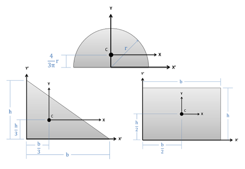
The location of centroids for a variety of common shapes can simply be looked up in tables, such as this table for 2D centroids and this table for 3D centroids. However, we will often need to determine the centroid of other shapes; to do this, we will generally use one of two methods.
- We can use the first moment integral to determine the centroid location.
- We can use the method of composite parts along with centroid tables to determine the centroid location.
On this page we will only discuss the first method, as the method of composite parts is discussed in a later section. The tables used in the method of composite parts, however, are derived via the first moment integral, so both methods ultimately rely on first moment integrals.
Finding the Centroid via the First Moment Integral
When we find the centroid of a two-dimensional shape, we will be looking for both an \(x\) and a \(y\) coordinate, represented as \(\bar{x}\) and \(\bar{y}\) respectively. Collectively, this \((\bar{x}, \bar{y}\) coordinate is the centroid of the shape.
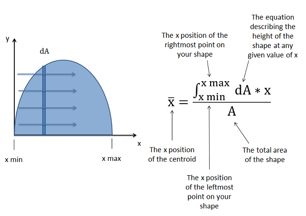
To find the average \(x\)-coordinate of a shape (\(\bar{x}\)), we will essentially break the shape into a large number of very small and equally sized areas, and find the average \(x\)-coordinate of these areas. To do this sum of an infinite number of very small things, we will use integration. Specifically, we will take the first rectangular area moment integral along the \(x\)-axis, and then divide that integral by the total area to find the average coordinate. We can do something similar along the \(y\)-axis to find our \(\bar{y}\) value. Writing all of this out, we have the equations below.
\[ C = ( \bar{x}, \bar{y}) \]
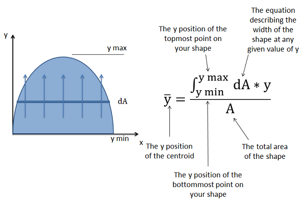
\begin{align} \bar{x} &= \dfrac{ \displaystyle\int_{A} (dA*x)}{A} \\[4pt] \bar{y} &= \dfrac{ \displaystyle\int_{A} (dA*y)}{A} \end{align}
Next let's discuss what the variable \(dA\) represents and how we integrate it over the area. The variable \(dA\) is the rate of change in area as we move in a particular direction. For \(\bar{x}\) we will be moving along the \(x\)-axis, and for \(\bar{y}\) we will be moving along the \(y\)-axis in these integrals.
As we move along the \(x\)-axis of a shape from its leftmost point to its rightmost point, the rate of change of the area at any instant in time will be equal to the height of the shape that point times the rate at which we are moving along the axis (\(dx\)). Because the height of the shape will change with position, we do not use any one value, but instead must come up with an equation that describes the height at any given value of x. We will then multiply this \(dA\) equation by the variable \(x\) (to make it a moment integral), and integrate that equation from the leftmost \(x\) position of the shape (\(x_{min}\)) to the rightmost \(x\) position of the shape (\(x_{max}\)).
To find the \(y\) coordinate of the of the centroid, we have a similar process, but because we are moving along the \(y\)-axis, the value \(dA\) is the equation describing the width of the shape times the rate at which we are moving along the \(y\) axis (\(dy\)). We then take this \(dA\) equation and multiply it by \(y\) to make it a moment integral. We will integrate this equation from the \(y\) position of the bottommost point on the shape (\(y_{min}\)) to the \(y\) position of the topmost point on the shape (\(y_{max}\)).
Using the first moment integral and the equations shown above, we can theoretically find the centroid of any shape as long as we can write out equations to describe the height and width at any \(x\) or \(y\) value respectively. For more complex shapes, however, determining these equations and then integrating these equations can become very time-consuming. That is why most of the time, engineers will instead use the method of composite parts or computer tools.
Using Symmetry as a Shortcut
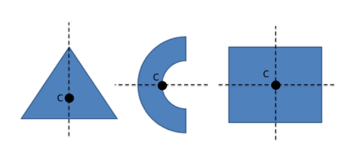
Shape symmetry can provide a shortcut in many centroid calculations. Remember that the centroid is located at the average \(x\) and \(y\) coordinate for all the points in the shape. If the shape has a line of symmetry, that means each point on one side of the line must have an equivalent point on the other side of the line. This means that the average value (AKA the centroid) must lie along any axis of symmetry. If the shape has more than one axis of symmetry, then the centroid must exist at the intersection of the two axes of symmetry.
Example \(\PageIndex{1}\)
Find the \(x\) and \(y\) coordinates of the centroid of the shape shown below.
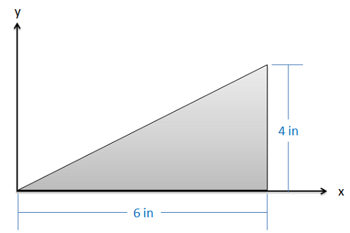
- Solution:
-
Video \(\PageIndex{2}\): Worked solution to example problem \(\PageIndex{1}\), provided by Dr. Jacob Moore. YouTube source: https://youtu.be/dZ2O3zwvuP0.
Example \(\PageIndex{2}\)
Find the \(x\) and \(y\) coordinates of the centroid of the shape shown below.
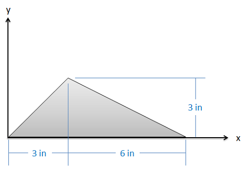
- Solution:
-
Video \(\PageIndex{3}\): Worked solution to example problem \(\PageIndex{2}\), provided by Dr. Jacob Moore. YouTube source: https://youtu.be/hmGiCFwgIo8.
Example \(\PageIndex{3}\)
Find the \(x\) and \(y\) coordinates of the centroid of the shape shown below.
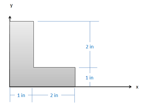
- Solution:
-
Video \(\PageIndex{4}\): Worked solution to example problem \(\PageIndex{3}\), provided by Dr. Jacob Moore. YouTube source: https://youtu.be/4MHflda4FBw.