9.5: Reactance and Impedance

Unlike a resistor, the voltage and current will not be in phase for an ideal capacitor or for an ideal inductor. For the capacitor, the current leads the voltage across the capacitor by 90 degrees. Recall that the voltage across a capacitor cannot change instantaneously, \(i = C \, dv/dt\). For an inductor, the voltage leads the current by 90 degrees. Similarly, the current through an inductor cannot change instantaneously due to \(v = L \, di/dt\). While ideal capacitors and inductors do not exhibit resistance, the voltage does react to the current. Unsurprisingly, we call this characteristic reactance and denote it with the letter \(X\). Reactance, like resistance, is a ratio of voltage to current. We define capacitive reactance as:

\[X_{C} = \frac{v_c}{i_c} \label{1.7} \]

Using a simple sine wave with a peak value of unity, \(v_c = \sin 2\pi f t\), \(i_c\) can be found from \(i = C \, dv/dt\). Recall from our prior work that the derivative or slope of a sine wave is a cosine wave, which is in turn equivalent to a sine wave shifted by +90\(^{\circ}\).

\[i_c = C \frac{dv_c}{dt} \nonumber \]

\[i_c = C \frac{d \sin(2 \pi f t)}{dt} \nonumber \]

\[i_c = C \sin (2 \pi f t+90^{\circ}) \nonumber \]

Substituting this result into Equation 1.7 yields:

\[X_C = \frac{v_c}{i_c} \nonumber \]

\[X_C = \frac{\sin (2 \pi f t)}{2 \pi f C \sin (2\pi f t+90^{\circ})} \nonumber \]

\[X_C = \frac{1}{2} \pi f C \angle −90^{\circ} \nonumber \]

Or more directly:

\[X_C =− j \frac{1}{2 \pi f C} \label{1.8} \]

In summation, if we divide the capacitor's sinusoidal voltage by its current (Ohm's law), we obtain a value with a phase angle of −90\(^{\circ}\). While the resultant is an ohmic value, it cannot be classified as a resistance. Instead, it is referred to as a reactance and denoted with the letter \(X\). Thus we can refer to a capacitor's reactance, \(X_C\), as some number at an angle of −90\(^{\circ}\), or more conveniently, we simply prepend \(−j\), as in \(X_C = −j75 \Omega\).

The case for the inductor is similar and left as an exercise. The inductive reactance, \(X_L\), can be found using:

\[X_L=+ j 2 \pi f L \label{1.9} \]

An example would be \(X_L = j68 \Omega\). As stated, while a resistance cannot be added directly to a reactance, reactances can be added together so long as we heed the signs. For example, if we have a capacitive reactance of \(−j60 \Omega\) in series with an inductive reactance of \(j100 \Omega\), the result is \(j40 \Omega\). This is due to the fact that these two items are 180 degrees out of phase with each other, and so they partially cancel. Remember, always add or subtract like items: real (resistance) to real, and imaginary (reactance) to imaginary.

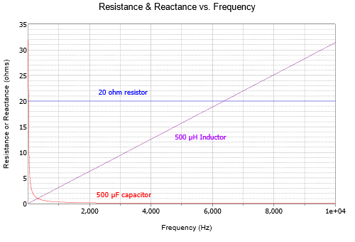
Equations \ref{1.8} and \ref{1.9} are notable because the reactance is not just a function of the capacitance or inductance, but also a function of frequency. The reactance of an inductor is directly proportional to frequency while the reactance of a capacitor is inversely proportional to frequency. The ohmic variations of a \(20 \Omega\) resistor, a 500 \(\mu\)F capacitor and a 500 \(\mu\)H inductor across frequency are shown in Figure \(\PageIndex{1}\).

We can see that the value of resistance does not change with frequency while the inductive reactance increases with frequency and the capacitive reactance decreases.

Figure \(\PageIndex{1}\): Resistance and reactance versus frequency (linear axis).

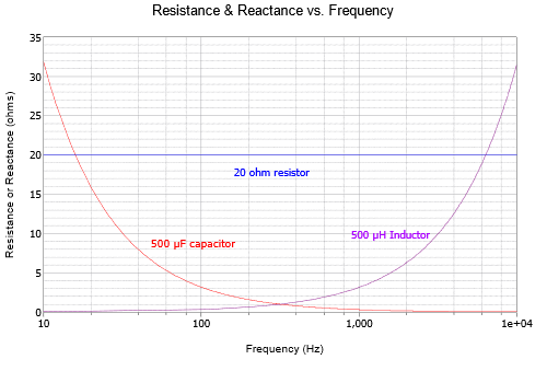
The linear frequency scale makes the capacitor change difficult to see. If this is plotted again but using a logarithmic frequency scale as in Figure \(\PageIndex{2}\), the symmetry becomes apparent.

Figure \(\PageIndex{2}\): Resistance and reactance versus frequency (log axis).

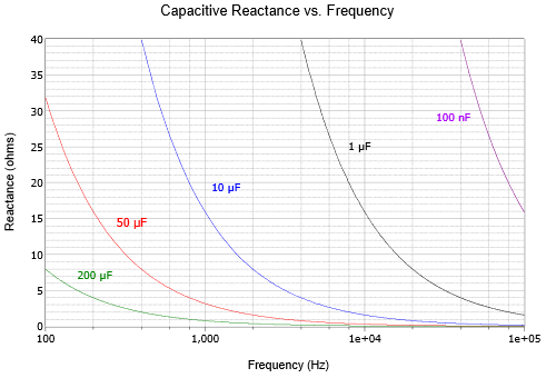
The effect of both capacitor size and frequency is shown in Figure \(\PageIndex{3}\) using a log frequency axis: the smaller the capacitor, the larger the capacitive reactance at any particular frequency.

Figure \(\PageIndex{3}\): Variation of capacitive reactance with capacitance and frequency.

Similarly, the effect of both inductor size and frequency is shown in Figure \(\PageIndex{4}\) using a linear frequency axis: the larger the inductor, the larger the inductive reactance at any given frequency.

Figure \(\PageIndex{4}\): Variation of inductive reactance with inductance and frequency.

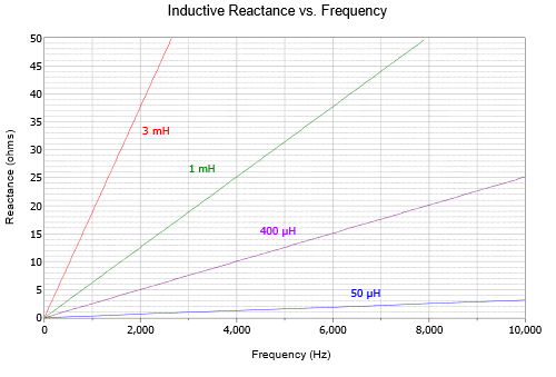
It is worth noting that the plots of Figures \(\PageIndex{3}\) and \(\PageIndex{4}\) are for ideal components. In reality, all components exhibit some resistive, capacitive and inductive effects due to their construction. For example, eventually, inductive and resistive effects will cause the capacitive reactance curves of Figure \(\PageIndex{3}\) to begin to rise at high frequencies. Similarly, resistive and capacitive effects will cause the curves Figure \(\PageIndex{4}\) to flatten at very low and very high frequencies.

An interesting observation to remember is that capacitors and inductors are a bit like a Chimera. That is, they look like different things to different sources, all mashed together at once. It would be improper to think of, say, a particular inductor as being “so many ohms”. If the source signal is comprised of multiple sine waves, such as a square wave or a music waveform, the inductor “looks like” a different ohmic value to each of the different frequency components, simultaneously. This is an important concept and one that we can take great advantage of, for example, in the design of filter circuits.

Impedance

We now arrive at impedance. Impedance is a mixture of resistance and reactance, and is denoted by \(Z\). This can be visualized as a series combination of a resistor and either a capacitor or an inductor. Examples include \(Z = 100 − j50 \Omega\), i.e., 100 ohms of resistance in series with 50 ohms of capacitive reactance; and \(Z = 600\angle 45^{\circ} \Omega\), i.e., a magnitude of 600 ohms that includes resistance and inductive reactance (it must be inductive reactance and not capacitive reactance because the sign of the angle is positive).

To complete this system, we have susceptance and admittance. Susceptance, \(S\), is the reciprocal of reactance. Admittance, \(Y\), is the reciprocal of impedance. These are similar to the relation between conductance and resistance, and are convenient for parallel circuit combinations.

Example \(\PageIndex{1}\)

Determine the reactances of a 1 mH inductor and a 2 \(\mu\)F capacitor to a sine wave of 2 kHz. Repeat for a frequency of 50 kHz.

Use Equations \ref{1.8} and \ref{1.9}. For the capacitor at 2 kHz we have:

\[X_C =− j \frac{1}{2\pi f C} \nonumber \]

\[X_C = − j \frac{1}{2 \pi 1kHz 2 \mu F} \nonumber \]

\[X_C =− j 79.6\Omega \nonumber \]

For the second source, 50 kHz is 25 times larger than the original and capacitive reactance is inversely proportional to frequency. Therefore \(X_C\) is 25 times smaller, or \(−j3.18 \Omega\).

For the inductor at 2 kHz,

\[X_L = +j 2\pi f L \nonumber \]

\[X_L = +j 2\pi 2 kHz 1 mH \nonumber \]

\[X L = +j 12.57\Omega \nonumber \]

Inductive reactance is directly proportional to frequency. Thus, increasing f by a factor of 25 increases \(X_L\) by the same factor, resulting in \(j314.2 \Omega\).

Example \(\PageIndex{2}\)

Determine the susceptance of an inductor whose reactance is \(j400 \Omega\). Further, if this inductor is placed in series with a \(1000 \Omega\) resistor, determine the resulting impedance in polar form, as well as the admittance.

Susceptance is the reciprocal of reactance.

\[S_L = \frac{1}{X_L} \nonumber \]

\[S_L = \frac{1}{j 400\Omega} \nonumber \]

\[S_L = − j 2.5 \text{ millisiemens} \nonumber \]

The impedance, \(Z\), is the vector sum, or \(1000 + j400 \Omega\). Converting this to polar form:

\[\text{Magnitude } = \sqrt{\text{Real}^2 + \text{Imaginary}^2} \nonumber \]

\[\text{Magnitude } = \sqrt{1000^2+400^2} \nonumber \]

\[\text{Magnitude } = 1077 \nonumber \]

\[\theta = \tan^{−1} \left( \frac{\text{Imaginary}}{\text{Real}} \right) \nonumber \]

\[\theta = \tan^{−1} \left( \frac{400}{1000} \right) \nonumber \]

\[\theta = 21.8^{\circ} \nonumber \]

The result is \(Z = 1077\angle 21.8^{\circ} \Omega\). The admittance is the reciprocal, yielding \(Y = 928E-6\angle −21.8^{\circ} \mu S\).