
17.4: Centroids and Centers of Mass via Method of Composite Parts
- Page ID
- 55341

\( \newcommand{\vecs}[1]{\overset { \scriptstyle \rightharpoonup} {\mathbf{#1}} } \)
\( \newcommand{\vecd}[1]{\overset{-\!-\!\rightharpoonup}{\vphantom{a}\smash {#1}}} \)
\( \newcommand{\dsum}{\displaystyle\sum\limits} \)
\( \newcommand{\dint}{\displaystyle\int\limits} \)
\( \newcommand{\dlim}{\displaystyle\lim\limits} \)
\( \newcommand{\id}{\mathrm{id}}\) \( \newcommand{\Span}{\mathrm{span}}\)
( \newcommand{\kernel}{\mathrm{null}\,}\) \( \newcommand{\range}{\mathrm{range}\,}\)
\( \newcommand{\RealPart}{\mathrm{Re}}\) \( \newcommand{\ImaginaryPart}{\mathrm{Im}}\)
\( \newcommand{\Argument}{\mathrm{Arg}}\) \( \newcommand{\norm}[1]{\| #1 \|}\)
\( \newcommand{\inner}[2]{\langle #1, #2 \rangle}\)
\( \newcommand{\Span}{\mathrm{span}}\)
\( \newcommand{\id}{\mathrm{id}}\)
\( \newcommand{\Span}{\mathrm{span}}\)
\( \newcommand{\kernel}{\mathrm{null}\,}\)
\( \newcommand{\range}{\mathrm{range}\,}\)
\( \newcommand{\RealPart}{\mathrm{Re}}\)
\( \newcommand{\ImaginaryPart}{\mathrm{Im}}\)
\( \newcommand{\Argument}{\mathrm{Arg}}\)
\( \newcommand{\norm}[1]{\| #1 \|}\)
\( \newcommand{\inner}[2]{\langle #1, #2 \rangle}\)
\( \newcommand{\Span}{\mathrm{span}}\) \( \newcommand{\AA}{\unicode[.8,0]{x212B}}\)
\( \newcommand{\vectorA}[1]{\vec{#1}} % arrow\)
\( \newcommand{\vectorAt}[1]{\vec{\text{#1}}} % arrow\)
\( \newcommand{\vectorB}[1]{\overset { \scriptstyle \rightharpoonup} {\mathbf{#1}} } \)
\( \newcommand{\vectorC}[1]{\textbf{#1}} \)
\( \newcommand{\vectorD}[1]{\overrightarrow{#1}} \)
\( \newcommand{\vectorDt}[1]{\overrightarrow{\text{#1}}} \)
\( \newcommand{\vectE}[1]{\overset{-\!-\!\rightharpoonup}{\vphantom{a}\smash{\mathbf {#1}}}} \)
\( \newcommand{\vecs}[1]{\overset { \scriptstyle \rightharpoonup} {\mathbf{#1}} } \)
\(\newcommand{\longvect}{\overrightarrow}\)
\( \newcommand{\vecd}[1]{\overset{-\!-\!\rightharpoonup}{\vphantom{a}\smash {#1}}} \)
\(\newcommand{\avec}{\mathbf a}\) \(\newcommand{\bvec}{\mathbf b}\) \(\newcommand{\cvec}{\mathbf c}\) \(\newcommand{\dvec}{\mathbf d}\) \(\newcommand{\dtil}{\widetilde{\mathbf d}}\) \(\newcommand{\evec}{\mathbf e}\) \(\newcommand{\fvec}{\mathbf f}\) \(\newcommand{\nvec}{\mathbf n}\) \(\newcommand{\pvec}{\mathbf p}\) \(\newcommand{\qvec}{\mathbf q}\) \(\newcommand{\svec}{\mathbf s}\) \(\newcommand{\tvec}{\mathbf t}\) \(\newcommand{\uvec}{\mathbf u}\) \(\newcommand{\vvec}{\mathbf v}\) \(\newcommand{\wvec}{\mathbf w}\) \(\newcommand{\xvec}{\mathbf x}\) \(\newcommand{\yvec}{\mathbf y}\) \(\newcommand{\zvec}{\mathbf z}\) \(\newcommand{\rvec}{\mathbf r}\) \(\newcommand{\mvec}{\mathbf m}\) \(\newcommand{\zerovec}{\mathbf 0}\) \(\newcommand{\onevec}{\mathbf 1}\) \(\newcommand{\real}{\mathbb R}\) \(\newcommand{\twovec}[2]{\left[\begin{array}{r}#1 \\ #2 \end{array}\right]}\) \(\newcommand{\ctwovec}[2]{\left[\begin{array}{c}#1 \\ #2 \end{array}\right]}\) \(\newcommand{\threevec}[3]{\left[\begin{array}{r}#1 \\ #2 \\ #3 \end{array}\right]}\) \(\newcommand{\cthreevec}[3]{\left[\begin{array}{c}#1 \\ #2 \\ #3 \end{array}\right]}\) \(\newcommand{\fourvec}[4]{\left[\begin{array}{r}#1 \\ #2 \\ #3 \\ #4 \end{array}\right]}\) \(\newcommand{\cfourvec}[4]{\left[\begin{array}{c}#1 \\ #2 \\ #3 \\ #4 \end{array}\right]}\) \(\newcommand{\fivevec}[5]{\left[\begin{array}{r}#1 \\ #2 \\ #3 \\ #4 \\ #5 \\ \end{array}\right]}\) \(\newcommand{\cfivevec}[5]{\left[\begin{array}{c}#1 \\ #2 \\ #3 \\ #4 \\ #5 \\ \end{array}\right]}\) \(\newcommand{\mattwo}[4]{\left[\begin{array}{rr}#1 \amp #2 \\ #3 \amp #4 \\ \end{array}\right]}\) \(\newcommand{\laspan}[1]{\text{Span}\{#1\}}\) \(\newcommand{\bcal}{\cal B}\) \(\newcommand{\ccal}{\cal C}\) \(\newcommand{\scal}{\cal S}\) \(\newcommand{\wcal}{\cal W}\) \(\newcommand{\ecal}{\cal E}\) \(\newcommand{\coords}[2]{\left\{#1\right\}_{#2}}\) \(\newcommand{\gray}[1]{\color{gray}{#1}}\) \(\newcommand{\lgray}[1]{\color{lightgray}{#1}}\) \(\newcommand{\rank}{\operatorname{rank}}\) \(\newcommand{\row}{\text{Row}}\) \(\newcommand{\col}{\text{Col}}\) \(\renewcommand{\row}{\text{Row}}\) \(\newcommand{\nul}{\text{Nul}}\) \(\newcommand{\var}{\text{Var}}\) \(\newcommand{\corr}{\text{corr}}\) \(\newcommand{\len}[1]{\left|#1\right|}\) \(\newcommand{\bbar}{\overline{\bvec}}\) \(\newcommand{\bhat}{\widehat{\bvec}}\) \(\newcommand{\bperp}{\bvec^\perp}\) \(\newcommand{\xhat}{\widehat{\xvec}}\) \(\newcommand{\vhat}{\widehat{\vvec}}\) \(\newcommand{\uhat}{\widehat{\uvec}}\) \(\newcommand{\what}{\widehat{\wvec}}\) \(\newcommand{\Sighat}{\widehat{\Sigma}}\) \(\newcommand{\lt}{<}\) \(\newcommand{\gt}{>}\) \(\newcommand{\amp}{&}\) \(\definecolor{fillinmathshade}{gray}{0.9}\)As an alternative to the use of moment integrals, we can use the Method of Composite Parts to find the centroid of an area or volume or the center of mass of a body. This method is is often easier and faster that the integration method; however, it will be limited by the table of centroids you have available. The method works by breaking the shape or volume down into a number of more basic shapes, identifying the centroids or centers of masses of each part via a table of values, and then combing the results to find the overall centroid or center of mass.
A key aspect of the method is the use of these centroid tables. This is a set of tables that lists the centroids (and usually also moments of inertia) for a number of common areas and/or volumes. Some centroid tables can be found here for 2D shapes, and here for 3D shapes. The method of composite parts is limited in that we will need to be able to break our complex shape down entirely into shapes found in the centroid table we have available; otherwise, the method will not work without us also doing some moment integrals.
Finding the Centroid via the Method of Composite Parts
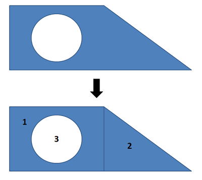
Start the process by labeling an origin point and axes on your shape. It will be important to measure all locations from the same point. Next, we must break our complex shape down into several simpler shapes. This may include areas or volumes (which we will count as positive areas or volumes) or holes (which we will count as negative areas or volumes). Each of these shapes will have a centroid (\(C\)) or center of mass (\(G\)) listed on the diagram.
Once we have identified the different parts, we will create a table listing the area or volume of each piece, and the \(x\) and \(y\) centroid coordinates (or \(x\), \(y\), and \(z\) coordinates in 3D). It is important to remember that each coordinate you list should be relative to the same base origin point that you drew in earlier. You may need to mentally adjust diagrams in the centroid tables so that the shape is oriented in the right direction, and account for the placement of the shape relative to the axes in your diagram.
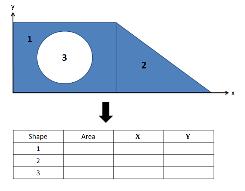
Once you have the areas and centroid coordinates for each shape relative to your origin point, you can find the \(x\) and \(y\) coordinate of the centroid for the overall shape with the following formulas. Remember that areas or volumes for any shape that is a hole or cutout in the design will be a negative area in your formula.
\[ \bar{x}_{total} = \frac{\sum A_i \bar{x}_i}{A_{total}} \quad\quad\quad \bar{y}_{total} = \frac{\sum A_i \bar{y}_i}{A_{total}} \]
This generalized formula to find the centroid's \(x\)-location is simply Area 1 times \(\bar{x}_1\), plus Area 2 times \(\bar{x}_2\), plus Area 3 times \(\bar{x}_3\), adding up as many shapes as you have in this fashion and then dividing by the overall area of your combined shape. The equations are the same for the \(y\)-location of the overall centroid, except you will instead be using \(\bar{y}\) values in your equations.
For centroids in three dimensions we will simply use volumes in place of areas, and we will have a \(z\) coordinate for our centroid as well as the \(x\) and \(y\) coordinates.
Finding the Center of Mass via the Method of Composite Parts
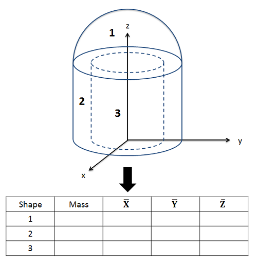
To use the method of composite parts to find the center of mass, we simply need to adjust the process slightly. First, center of mass calculations will always be in three dimensions. Draw an origin point and some axes on your diagram we did for the centroid. We will measure all locations relative to this origin point. We will then need to break the complex shape down into simple volumes, with each simple volume being something in the centroid table we have available. Remember that when we have a part with a uniform material, the centroid and center of mass are the same point, so we will often talk about these interchangeably.
Once we have identified the different parts, we will create a table indicating the mass of each part, and the x, y, and z coordinate of the center of mass for each individual part. It is important to remember that each coordinate you list should be relative to the same base origin point, so you will need to mentally rotate and position the parts in the table on your axes.
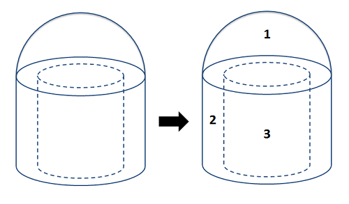
One complicating factor with mass can be measuring the mass of the pieces separately. If we have a scale, we may simply know the overall mass without knowing the mass of the individual pieces. In these cases, you may need work backwards to calculate the density of the material (by dividing the overall mass by overall volume), and then use density times piece volume to find the mass of each piece individually. When doing this, remember to count cutouts as negative mass in your calculations. For example, for the hollow cylinder in the shape above, you would find the mass of a solid cylinder for Shape 2, then have a negative mass for the cylindrical cutout for Shape 3.
Finally, once you have the mass the and center of mass coordinates for each shape, you can find the coordinates of the center of mass for the overall volume with the following formulas.
\[ x_G = \frac{\sum m_i \bar{x}_i}{m_{total}} \quad\quad y_G = \frac{\sum m_i \bar{y}_i}{m_{total}} \quad\quad z_G = \frac{\sum m_i \bar{z}_i}{m_{total}} \]
Similar to the centroid equations, the \(x\)-equation is simply the mass of Shape 1 times \(\bar{x}_1\), plus the mass of Shape 2 times \(\bar{x}_2\), and so on for each part. After you have summed up these products for all the shapes, just divide by the total mass.
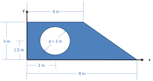
Example \(\PageIndex{1}\)
Find the \(x\) and \(y\) coordinates of the centroid of the shape shown below.
- Solution:
-
Video \(\PageIndex{2}\): Worked solution to example problem \(\PageIndex{2}\), provided by Dr. Jacob Moore. YouTube source: https://youtu.be/QIe6Hk4Bofs.
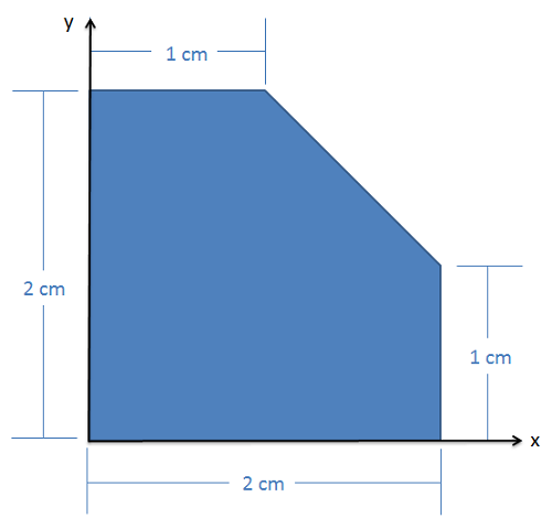
Example \(\PageIndex{2}\)
Find the \(x\) and \(y\) coordinates of the centroid of the shape shown below.
- Solution:
-
Video \(\PageIndex{3}\): Worked solution to example problem \(\PageIndex{2}\), provided by Dr. Jacob Moore. YouTube source: https://youtu.be/F1rlzboPlZM.
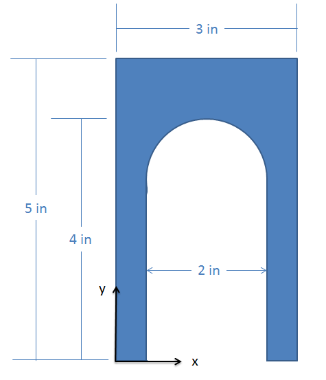
Example \(\PageIndex{3}\)
Find the \(x\) and \(y\) coordinates of the centroid of the shape shown below.
- Solution:
-
Video \(\PageIndex{4}\): Worked solution to example problem \(\PageIndex{3}\), provided by Dr. Jacob Moore. YouTube source: https://youtu.be/tLybTEX8S_I.
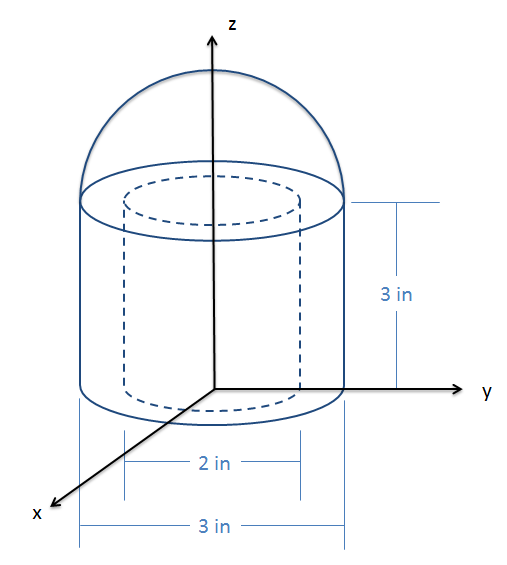
Example \(\PageIndex{4}\)
The shape shown below consists of a solid semicircular hemisphere on top of a hollow cylinder. Based on the dimensions below, determine the location of the centroid.
- Solution:
-
Video \(\PageIndex{5}\): Worked solution to example problem \(\PageIndex{4}\), provided by Dr. Jacob Moore. YouTube source: https://youtu.be/vQk4OqTcDpQ.
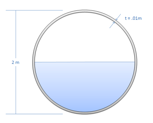
Example \(\PageIndex{5}\)
A spherical steel tank (density = 8050 kg/m3) is filled halfway with water (density = 1000 kg/m3) as shown below. Find the overall mass of the tank and the current location of the center of mass of the tank (measured from the base of the tank).
- Solution:
-
Video \(\PageIndex{6}\): Worked solution to example problem \(\PageIndex{5}\), provided by Dr. Jacob Moore. YouTube source: https://youtu.be/5zbYD4Wogck.